Taylor Expansion
A straight line used one slope to estimate a nearby value. Now we want to keep more of the way a function changes, without losing the simple calculations of a polynomial.
Return to Approximation01What could improve the straight line?
In Approximation, we started from a value we knew and used the slope there to estimate a nearby value. The known starting input was called there; here we will call it . The target input is , and is the signed change from to . A negative means that the target lies to the left.
The value fixes where the line passes. The derivative fixes its direction. However, a line keeps the same slope everywhere, while the function may turn gradually. To follow that change, we need more than a term proportional to .
Why look for a polynomial? An expression such as only asks us to multiply and add, making it easier to evaluate than square roots or trigonometric values. The question is how to choose its coefficients for a reason.
02Choose a centre, then say what should match
Let us first choose , where a positive integer power of zero is zero. A polynomial is a finite sum of powers: a constant, a multiple of , a multiple of . The numbers multiplying those powers are the coefficients , where the subscript records the power.
names the polynomial we are building, and is the highest power we keep. The constant contains no at all. We will choose these coefficients so that and agree at zero, and then ask their derivatives to agree there too.
The first condition makes the graphs pass through the same point. The second, when , gives them the same slope at that point. These are exactly the two jobs that the tangent line did.
Differentiating gives f''', the third derivative. If we retain powers through , we match derivatives through order at zero.
This is a construction rule for a finite polynomial. We have not said that the two functions are equal away from zero; how close they are is tested below.
03Make one unknown coefficient the only survivor
Start with . Putting removes every term containing a positive power of , leaving , so . To find in the same way, differentiate once to make it a constant: becomes .
A constant has derivative zero because it does not change. Differentiating brings down as a multiplier and lowers the power to ; multiplying the term by fixed multiplies its derivative by .
Why does the exponent become a multiplier?
For a positive integer n, (x+t)ⁿ is a product of n identical brackets. When we multiply them out, the term containing no t is xⁿ. A term containing exactly one t is formed by choosing t from one bracket and x from all the others. There are n choices of that bracket, so these terms add to nxⁿ⁻¹t. Every other contribution contains at least two factors t.
B(t) is just a name for the finite polynomial left after taking t² out of the remaining terms. Keep t nonzero while dividing by it. Then let t approach zero; the part tB(t) tends to zero because B(t) stays finite near zero. The remaining slope is nxⁿ⁻¹.
The symbol d/dx means “differentiate with respect to x”. For n = 0, the term is the constant 1 and its derivative is 0; we do not use the displayed positive-power formula to create a negative power there.
Find one coefficient, keeping its history
Choose a coefficient. Use Next to inspect every differentiation before substituting zero. The small original-term label shows where each term came from.
Try . After two derivatives its term is . Then substituting removes higher powers, while lower powers have already disappeared through differentiation. Thus , giving . For , division by removes those extra factors.
It reaches a constant sooner. The next derivative turns that constant into zero.
It has just reached a constant. It is the term we keep.
It still contains x. Substituting zero removes it.
04Keep the pattern, without skipping the factors
After derivatives of , no remains and the multiplier is . That product is called factorial, written . Therefore , giving .
The notation means differentiating times. For the constant term we use conventions and , making the same rule give .
The large means “add”. stays fixed while counts from to . Built around zero, this polynomial is called a Maclaurin polynomial.
If one derivative is zero, its coefficient is zero too. We keep the matching rule even when a term contributes nothing.
05Try a function whose answer we can check
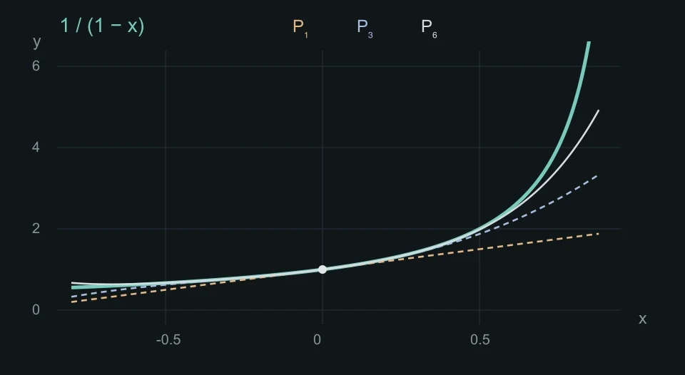
Before trusting the method for a difficult calculation, choose , where division lets us check values independently: . The input is not allowed because its denominator would be zero.
Taking one difference quotient gives derivative .
Continue to every derivative, without a memorized rule
Write b=1−x temporarily. For a positive integer m, the change of (1−x)⁻ᵐ has numerator bᵐ−(b−t)ᵐ after bringing the two fractions to a common denominator. The finite-product argument from the power rule gives bᵐ−(b−t)ᵐ=mbᵐ⁻¹t+t²C(t), where C is a finite polynomial. Divide by t and let t approach zero; b is nonzero because x≠1.
Thus differentiating (1−x)⁻ᵐ multiplies by m and increases the denominator power by one. Starting with m=1, the successive front factors are 1, then 1·2, then 1·2·3. Repeating the same step gives the general expression. At zero, the denominator is 1, so the derivative value is n!.
Each coefficient is therefore 1. The polynomials start as . At , and while exact is 2. The vertical difference is the error.
Keep x fixed; add one power at a time
is the highest power we keep. Change first and watch the dashed curve and the error reading. Then change to ask whether the same polynomial works farther from zero.
Where this polynomial value comes from
Add those contributions to get . The error is the absolute difference , so its sign does not matter here.
06What is left over, and may we keep going forever?
Call the finite sum by . We find its exact difference from the function by multiplying and subtracting; no general remainder formula is needed.
Subtract two almost identical sums
The first row is . Multiplying it by raises every power by one, giving the second row. Now subtract the second row from the first; each column keeps one power aligned.
The cancellation gives . Since , divide both sides by . The function is the finite polynomial plus exactly what is missing.
That missing part is called the remainder: . Unlike an approximation sign, this equation is exact for every finite and . For and , remainder is , accounting for the full gap.
Now keep fixed and increase . If , the magnitude tends to zero, so the remainder tends to zero. At , however, keeps alternating. Being a valid input is not enough to make the series approach .
Why do powers of a number between 0 and 1 tend to zero?
Call that number q, and let the positive integer m count how many factors q we multiply. If q=0 the claim is immediate. If 0<q<1, write 1/q=1+r with r>0. Expanding (1+r)ᵐ gives 1+mr plus further nonnegative terms, so it is at least 1+mr. Taking reciprocals gives 0<qᵐ≤1/(1+mr). The right side can be made smaller than any chosen positive amount by increasing m. Therefore qᵐ tends to zero.
Only after checking this limiting step may we write an infinite-series equality. The resulting infinite sum about zero is called the Maclaurin series. The symbol means the limit of the finite sums, not a calculation with an infinitely large .
For another function, matching derivatives still constructs its finite polynomial. It does not by itself prove that adding terms forever gives the function. We must check that function’s remainder as well.
07Move the centre without changing the function
Zero was convenient because substitution removed positive powers. Suppose we want and know values and derivatives at . The target is only away. We can treat as our new local zero.
The original input still names the same place. The new input tells how far, with a sign, that place lies from . We give this new input rule a name: , so .
Move the zero, keeping Q in place
First move , the expansion centre. keeps the same coordinate and height; only its local coordinate changes. The lower axis measures from instead of from zero.
Because an increase in is the same increase in , : derivatives at local zero are derivatives at .
Build the polynomial for , replace by , and replace by . The resulting polynomial is called the Taylor polynomial about ; Maclaurin is the special case .
The last line defines exactly. The quantity being approximated is , because . Writing would change the input.
Return to . The derivative formula gives coefficients . Since , the cubic approximation is .
The checked value is , so error is . Expanding about zero gives error . Moving the centre closer helps substantially.
Check the shifted remainder using the same finite sum
Factor 1−a out of the denominator. Call h/(1−a) by r; this is only a shorter name, and a≠1. The function becomes 1/(1−a) times 1/(1−r). Apply the exact finite-sum identity already derived, now with r in place of x.
First identify the finite polynomial part. Each power rⁿ is hⁿ/(1−a)ⁿ. The outside factor 1/(1−a) adds one more factor to the denominator. These are exactly the coefficients f⁽ⁿ⁾(a)/n! already found, so this finite sum is T_N(x).
The remaining term also has the outside factor 1/(1−a). Since (1−a)(1−r)=1−a−h=1−x, its denominator simplifies as follows.
The remainder tends to zero when .
The Taylor series is the infinite sum about . It equals only when the difference tends to zero: .
When checked at the chosen input, we may replace approximation by equality.
08Use the construction, then explain your choices
1 · If f(0)=2, f′(0)=−1 and f″(0)=6, what is P₂(x)?
The constant is ; the linear coefficient is . For the quadratic term, two derivatives introduce , so its coefficient is . Thus .
2 · For 1/(1−x), find P₃(0.2) and the exact remaining error.
The exact value is . The remainder formula gives , exactly the missing amount.
3 · If a=0.5 and x=0.4, what are h and g(h)?
. Negative sign places target to the left. , not .
Matching derivatives told us how to choose a finite polynomial; checking the remainder told us whether continuing to add terms was justified; moving the centre reused the construction with a new coordinate.
Back to mathematics