Approximation

01What is missing from “about 3”?

A square root reverses squaring: because $3^2=9$ , the nonnegative number whose square is 9 is 3. That gives us $\sqrt{9}=3$ exactly. Now increase the number under the root a little, from 9 to 9.1. Its square root also increases a little. So 3 is a useful first guess, but it misses that increase.

Can we estimate how much to add to 3, without already knowing $\sqrt{9.1}$ ? This is the need for an approximation: replace a harder calculation by an easier one, while keeping track of the difference we introduce. We write $\approx$ for “approximately equal”; it does not mean the two numbers are exactly equal.

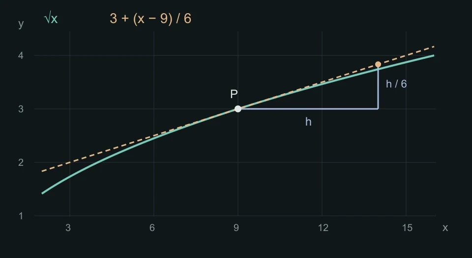
Let $f(x)=\sqrt{x}$ . Here $x$ is the input, and $f(x)$ is the output, drawn as the height of the curve. We know the point $P=(9,3)$ . We want the height of a nearby point $Q$ whose input is 9.1. Keeping the starting height 3 is our first guess. Our next guess will also use the slope at P.

02Keep the starting point. Name the change.

We will try several nearby inputs, so let us give the input change a name: $h$ . It is the new input minus the known input. Starting at 9, the new input is therefore $9+h$ . To reach 9.1, we need $h=9.1-9=0.1$ . To reach 8.9, we instead need $h=8.9-9=-0.1$ .

h=x-9,\qquad x=9+h

$h$ includes direction. Positive means move right; negative means move left. The distance is $|h|$ , the size of the change after removing its sign. Do not replace a negative $h$ by a positive distance in the calculation.

The height changes too, but usually by a different amount. It starts at $f(9)=3$ and ends at $f(9+h)$ . The height change is therefore $f(9+h)-3$ . The path from P to Q has two parts: a horizontal move of $h$ , followed by a vertical move to Q. The horizontal part records the input change; the vertical part records the output change. Try positive and negative $h$ , and compare these with $h=0$ .

True curve

The computer draws the true curve so we can check our work. Our approximation will use only the known point and its slope, not the unknown height at Q.

We still do not know the height change when we are doing the approximation ourselves. The diagram can calculate it for checking, but our method must predict it from information at P. What connects a horizontal change to a vertical change? The slope does.

03Use a slope we already know

For a straight line, slope means height change divided by input change. A slope of 2, for example, means that moving 1 unit to the right changes the height by 2 units. Multiplying a horizontal change by the slope gives the corresponding height change.

The square-root graph is curved, so one slope does not describe the whole graph. Join P and a different point Q with a straight line. This is the secant through those two points. As Q moves towards P, the secant slope approaches the slope at P. The line through P with that limiting slope is the tangent.

\text{secant slope}=\frac{f(9+h)-f(9)}{h},\qquad h\ne0

This limiting slope is the derivative at 9, written $f'(9)$ . The prime mark means “derivative”, not a new input. The limit below means that we examine smaller and smaller nonzero changes $h$ , from either side. It does not mean putting zero into the denominator.

f'(9)=\lim_{h\to0}\frac{f(9+h)-f(9)}{h}

The next section will calculate this slope as $1/6$ . For now, compare it with the secant slope. Let Q approach from either side, pause while the two slopes still differ, and zoom near P. Then try exactly $h=0$ : P and Q coincide, so the quotient is undefined, while the tangent slope still exists.

True curveTangent at PSecant through P and Q

Playback begins at |h| = 0.8 and stops at 0.001. It illustrates approaching zero; it does not claim to finish an infinite limiting process.

If $h$ is small but not zero, the secant slope is close to $f'(9)$ , rather than guaranteed to equal it. This is exactly where an approximation enters: we use the known tangent slope in place of the harder secant slope, and later check the error.

04Where does the slope 1/6 come from?

Let us calculate the slope, rather than treat it as a rule to remember. Substitute $f(x)=\sqrt{x}$ and $f(9)=3$ into the secant quotient. We assume $h\ne0$ while calculating it, and $9+h\ge0$ so the square root is defined.

\frac{f(9+h)-f(9)}{h}=\frac{\sqrt{9+h}-3}{h}

Remove the difference of roots

Both numerator and denominator become small near $h=0$ , so direct substitution would give $0/0$ . To see what cancels before taking the limit, use $(a-b)(a+b)=a^2-b^2$ . The opposite middle terms cancel when we expand the product. Here choose $a=\sqrt{9+h}$ and $b=3$ .

\begin{aligned}&(\sqrt{9+h}-3)(\sqrt{9+h}+3)\\&=(9+h)-9=h\end{aligned}

Multiply the fraction by $(\sqrt{9+h}+3)/(\sqrt{9+h}+3)$ . Its numerator and denominator are equal and positive, so this factor is 1: it changes the form, not the value.

\frac{\sqrt{9+h}-3}{h}=\frac{h}{h(\sqrt{9+h}+3)}

Cancel first. Take the limit afterwards.

Because $h$ is not zero, we can divide numerator and denominator by $h$ . The resulting denominator approaches $3+3=6$ as $h$ approaches zero. It stays away from zero, so the reciprocal approaches $1/6$ .

\frac{\sqrt{9+h}-3}{h}=\frac{1}{\sqrt{9+h}+3}\quad(h\ne0)

f'(9)=\lim_{h\to0}\frac{1}{\sqrt{9+h}+3}=\frac16

Notice the distinction: the simplified expression is defined at zero, but the original secant quotient is not. We used the simplified expression to find the limit of the original quotient. We did not make division by zero valid.

The same steps work at any positive starting input $u$ . Here $u$ is just a name for the known input, replacing our particular choice 9. Replace 3 by $\sqrt{u}$ in the calculation. The two roots in the denominator both approach $\sqrt{u}$ , so:

\begin{aligned}f'(u)&=\lim_{h\to0}\frac{1}{\sqrt{u+h}+\sqrt{u}}\\&=\frac{1}{2\sqrt{u}},\quad u>0\end{aligned}

05Turn the slope into a predicted height

Return to the original question: estimate the height near $P=(9,3)$ . We now know the tangent slope, $f'(9)=1/6$ . For a small nonzero $h$ , use this known slope in place of the secant slope. Then undo the division by $h$ and undo the subtraction of 3. Each algebra step has a movement in the diagram.

\frac{f(9+h)-3}{h}\approx f'(9)=\frac16

First multiply by $h$ . The left side becomes the height change. On the right, input change times slope gives our predicted height change. If $h$ is negative, this predicted change is negative too: we move down, not up.

f(9+h)-3\approx h\cdot\frac16

This is only the change. To get the final height, add back the starting height 3. Call the resulting point on the tangent T. It has the same input as Q, but T gives the predicted height and Q gives the true height.

f(9+h)\approx 3+\frac{h}{6}

Watch the construction before comparing the answers. Move horizontally by $h$ , change height by $h/6$ , then combine that change with 3. Use “Next step” to inspect one operation at a time. At $h=0$ there is no change and the result is exactly 3, without using a secant quotient.

True curveTangent at P

Inspect any moment1/4 · Move across by h

Known starting height3

Predicted height changeNext: h × 1/6

Starting height + changeAdd after the rise

The predicted value will appear after we combine the starting height and the change. You can pause during either movement.

The view is centred on this chosen step so a small rise remains visible. It stays fixed throughout playback. The dashed tangent supplies the prediction; the curve supplies the later check.

For the original target 9.1, the signed step is $h=0.1$ . Our prediction is:

\sqrt{9.1}\approx 3+0.1\cdot\frac16=3.016666\ldots

A more accurate calculation gives $\sqrt{9.1}\approx3.0166206258$ . The prediction differs by about $0.00004604$ , much less than the roughly $0.01662$ missed by simply saying 3. It is a better approximation in this example, but it is still an approximation. Let us inspect the remaining gap.

06See the error, even when it is small

Let $L$ denote the predicted height on the line. Define the signed error as $E=L-f(u+h)$ : prediction minus true value. A positive error means the prediction is too high; a negative error means it is too low. The absolute error $|E|$ keeps only the size. Here $u$ is the known starting input and $h$ is still target minus starting input.

On the full graph, Q and T can appear to overlap. That does not prove their values are equal: the gap may simply be smaller than a screen pixel. The separate window below magnifies only their vertical difference. It labels its scale and keeps that scale fixed while you change $h$ .

True curveTangent at P

Vertical gap at the same input x = 9.1

This shows only the small vertical difference, not the full height from zero. The scale stays fixed while h changes, so a smaller gap really appears smaller.

Signed step h (the magnifier scale stays fixed)0.1

True height at Q3.0166206258

Predicted height at T3.0166666667

Error: prediction − true+0.0000460409

Try h = 0.1, then 0.01, then 0.001 without changing the scale. The gap shrinks rapidly. Fit the last gap only afterwards, and read the new axis numbers: magnifying an error does not make the error larger. Then try the negative steps.

Why is this square-root prediction above the curve?

A few trials suggest this, but trials alone do not prove it for every allowed input. We can check the difference directly. To keep the algebra readable, give the two heights short names: $s=\sqrt{u}$ is the known starting height, and $r=\sqrt{u+h}$ is the true target height. Thus $s>0$ , $r\ge0$ , and $h=r^2-s^2$ .

The slope is $1/(2s)$ , so the prediction is $L=s+h/(2s)$ . Subtract the true height $r$ . Then multiply by the positive number $2s$ to remove the fraction:

E=s+\frac{h}{2s}-r,\qquad 2sE=2s^2+h-2sr

Now replace $h$ by $r^2-s^2$ . The remaining three terms form a square:

2sE=s^2+r^2-2sr=(r-s)^2

E=\frac{(r-s)^2}{2s}\ge0

The numerator is a square and the denominator is positive. Therefore the prediction cannot be below the square-root curve. It equals the true value when $h=0$ and is above it for every other allowed $h$ . This argument covers steps to the left as well as steps to the right.

Connect the gap to the size of the input change

We also have $h=r^2-s^2=(r-s)(r+s)$ . Because $r+s>0$ , this gives $r-s=h/(r+s)$ . Substitute it into the error formula and replace the short names by the heights they represent:

E=\frac{h^2}{2\sqrt{u}(\sqrt{u+h}+\sqrt{u})^2}

For a fixed positive $u$ and small $h$ , the denominator stays close to the positive number $8u\sqrt{u}$ . Meanwhile the numerator is $h^2$ . This explains the rapidly shrinking gap: making a small $h$ ten times smaller makes its square one hundred times smaller, while the denominator changes only a little. This is a local comparison, not an exact error ratio for arbitrary large steps.

The direction of the error depends on the function. For example, take $g(x)=x^2$ at the input 3. Expanding gives $(3+h)^2=9+6h+h^2$ . For nonzero $h$ , its secant slope is $((3+h)^2-9)/h=6+h$ , which tends to 6. Its tangent therefore predicts $9+6h$ . Prediction minus true value is $-h^2$ : this time the prediction is below the curve. “A tangent always overestimates” would be the wrong conclusion.

07Keep the method. Change the function.

Our construction used three pieces of information: a known input, its height, and the slope there. For a general function $f$ , call the known input $u$ . The known height is $f(u)$ and the derivative there is $f'(u)$ . To reach a nearby input $u+h$ , multiply the signed input change $h$ by the slope and add that height change to the starting height:

f(u+h)\approx f(u)+hf'(u)

Once $u$ is chosen, $f(u)$ and $f'(u)$ are fixed numbers. Only $h$ changes. The expression on the right is a straight-line rule: starting value plus a constant times the input change. Using this line to approximate the function near $u$ is called linearization. It is the same run-and-rise construction we just watched, now written for any suitable function.

You may also see the new input written as $x$ rather than $u+h$ . Then $h=x-u$ , so the predicted value is written $L(x)=f(u)+(x-u)f'(u)$ . This is not a second method: it names the target input directly instead of naming the change.

L(x)=f(u)+(x-u)f'(u)

There are conditions to check. The function must have a finite derivative at the chosen input, and the target must belong to its domain, the set of inputs for which it is defined. Merely having both function values is not enough. For $f(x)=\sqrt{x}$ , the value at zero exists, but the finite slope used here does not; that is why our square-root construction requires $u>0$ .

Having a derivative guarantees the straight-line prediction becomes locally accurate as the step becomes small: the remaining error divided by $|h|$ tends to zero. It does not tell us that a particular step is small enough for the precision we need. For our square-root example we derived an exact error formula. For another function, a numerical check or a separate error bound may be needed.

Why does the derivative give that guarantee? Write the prediction error as $E=f(u)+hf'(u)-f(u+h)$ . For a nonzero $h$ , divide by $h$ . What remains is the difference between the derivative and the secant slope:

\frac{E}{h}=f'(u)-\frac{f(u+h)-f(u)}{h}\longrightarrow 0

The secant slope approaches the derivative by its definition, so their difference tends to zero. Taking the absolute value gives $|E|/|h|\to0$ . This explains why the prediction improves locally. It also shows why we needed the derivative to exist in the first place.

08Build a prediction yourself

Keep the three roles separate: $f(u)$ is a height, $h$ is a signed input change, and $f'(u)$ is height change per unit input. Multiplying the last two gives a height change, not a final height. Only after adding $f(u)$ do we have the predicted answer. Try a step to the right and a step to the left.

Use the known input $u=4$ , where $f(u)=2$ . Find the signed input change first. Then multiply it by the slope $1/(2\sqrt{u})$ , and add the starting height. What prediction do you get?

Your predicted value

A straight line keeps the height and slope at the chosen point, but it cannot bend with the curve. If we want a better approximation over a wider interval, we need a rule that can also match how the slope changes. The next page builds that idea step by step with Maclaurin and Taylor polynomials.