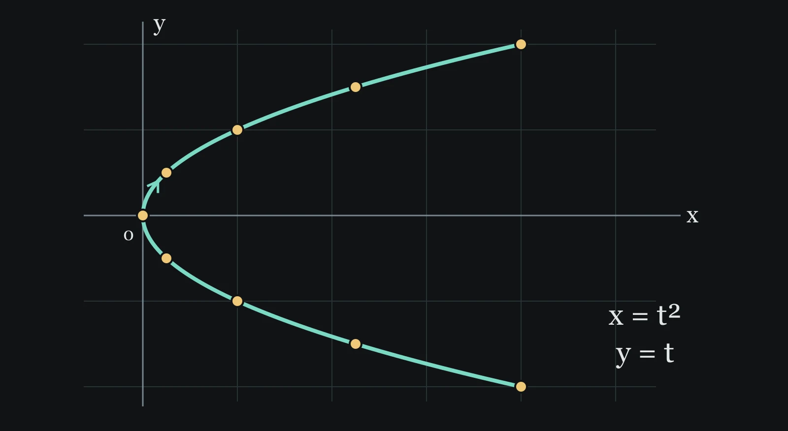
Parametric equations

01Why not always write $y$ as a function of $x$ ?

A function $y=f(x)$ assigns exactly one $y$ to each allowed $x$ . For example, $y=x^{2}$ assigns $y=4$ to $x=2$ . Now turn that relation around and ask for all points satisfying $x=y^{2}$ . When $x=4$ , both $y=2$ and $y=-2$ work, because $2^{2}=4$ and $(-2)^{2}=4$ . One rule $y=f(x)$ cannot return both heights at that same $x$ . The curve is still perfectly meaningful; this particular way of describing it is too restrictive.

For this curve, we can choose the vertical coordinate first. Call our chosen number $t$ . Set $y=t$ , and the relation $x=y^{2}$ then gives $x=t^{2}$ . If $t=-2$ , we get $(4,-2)$ ; if $t=2$ , we get (4,2). We have kept both points by allowing different values of $t$ to produce the same $x$ .

\begin{cases}x=t^2\\y=t\end{cases}\qquad t\longmapsto (t^2,t)

The extra number that labels our position along a curve is called a parameter. The letter $t$ is only a choice of name: here it is the chosen vertical coordinate, not time and not a third spatial direction. A pair of rules $x=f(t), y=g(t)$ means: choose one $t$ , put that same $t$ into each rule, and use the two results as one point. The names $f$ and $g$ can differ because the two calculations can differ. The input must stay the same so that we know which $x$ belongs with which $y$ .

This notation does not claim that every curve can be recovered from a single-valued $y=f(x)$ , or that each point has only one parameter value. It is a way to specify a path whenever we can give two coordinate rules and a range for their shared parameter. An ordinary function is included: choose $x=t$ and $y=f(t)$ . Giving a parameter range matters, because $-2\le t\le 2$ describes only the displayed piece of $x=y^{2}$ , not its infinite continuation.

02From one table row to one point

We will keep $x=t^{2}$ and $y=t$ for the first construction. For $t=-1.5$ , calculate $x=(-1.5)\times (-1.5)=2.25$ and $y=-1.5$ , so the point is $(2.25,-1.5)$ . On the graph, move right to $x=2.25$ , then down to $y=-1.5$ . These two moves locate the point; they are a plotting procedure, not the curve’s actual route between samples.

Press “Next step” to calculate, move horizontally, and then move vertically. The gold mark follows the current row; the teal points stay where they were placed. “Plot the points” repeats those steps and can be paused. The construction slider and row buttons let you inspect any step without the lesson advancing. Keep the sideways parabola selected first; we will explain the circle option just below.

Gold: current constructionTeal: points already retained

Choose a row to inspect its calculation. Decimal values are rounded.
$t$	$x$	$y$
-2	4	-2
-1.5	2.25	-1.5
-1	1	-1
-0.5	0.25	-0.5
0	0	0
0.5	0.25	0.5
1	1	1
1.5	2.25	1.5
2	4	2

Coordinate rules

x=t^2,\quad y=t,\quad -2\leq t\leq2

t = -2; x = (-2)² = 4; y = -2

First calculate both coordinates using this one value of $t$ . The gold table row is the pair we will plot next.

Construction step0

After all nine rows, we still have only nine points. To draw between them, we must keep using $x=t^{2}$ and $y=t$ for intermediate $t$ values. Eliminating $t$ confirms the shape: $y=t$ gives $t=y$ , and substituting into $x=t^{2}$ gives $x=y^{2}$ . Conversely, every point of $x=y^{2}$ with $-2\le y\le 2$ is obtained by choosing $t=y$ . This two-way argument identifies the whole piece of curve; a finite plot alone would not do that.

03The same idea draws a circle

A circle has the same difficulty with $y=f(x)$ : at $x=0$ , a circle of radius 2 centred at the origin has $y=2$ and $y=-2$ . An angle gives us a more useful label. Measure $t$ anticlockwise from the positive x-axis in radians. A radian measures arc length divided by radius; one whole turn is $2\pi$ radians. On the unit circle, cosine is defined as the horizontal coordinate and sine as the vertical coordinate. Scaling both coordinates by 2 therefore puts the point on the circle of radius 2.

x=2\cos t,\quad y=2\sin t,\quad 0\le t\le 2\pi

Here is why the radius stays fixed. On the unit circle, the right triangle made by the horizontal and vertical coordinates has hypotenuse 1. Pythagoras gives $\cos ^{2}t+\sin ^{2}t=1$ . Squaring signed coordinates makes the same calculation valid in every quadrant. Our new coordinates therefore satisfy $x^{2}+y^{2}=4\cos ^{2}t+4\sin ^{2}t=4$ . Their distance from the origin is $\sqrt{4}=2$ . As $t$ makes one full turn, every direction occurs, so we get every point on that circle.

To see the right triangle, choose the circle, inspect table row 2 and press ‘Next step’ twice. The horizontal and vertical gold segments are its perpendicular sides; the line back to the origin is its radius. The distance calculation below also explains the Pythagorean rule we just used.

Derive the distance rule used above

Take a right triangle with perpendicular lengths $a$ and $b$ and sloping side $c$ . Four identical copies fit inside the large square below, leaving a smaller square whose sides are $c$ . Each corner of the smaller square is a right angle because the two acute angles of a right triangle add to 90°. A rectangle of sides $a$ and $b$ is cut by a diagonal into two equal triangles, so each triangle has area $ab/2$ .

\begin{gathered}(a+b)^2=4\cdot\frac{ab}{2}+c^2\\a^2+2ab+b^2=2ab+c^2\\a^2+b^2=c^2\end{gathered}

The large area equals the four triangle areas plus the inner square. Expanding $(a+b)^{2}$ and subtracting $2ab$ from both sides gives $a^{2}+b^{2}=c^{2}$ . For coordinates x,y, the perpendicular lengths are |x| and |y|; squaring removes their signs, so the squared distance is $x^{2}+y^{2}$ . This is why the circle calculation works in every quadrant.

Now choose the circle in the plot. At $t=0$ , the radius points right, giving (2,0); at $\pi /2$ it points up, giving (0,2); at $\pi$ it points left, giving $(-2,0)$ ; at $3\pi /2$ it points down, giving $(0,-2)$ ; at $2\pi$ it returns to (2,0). Halfway through each quarter turn, the two perpendicular distances are equal. If either unsigned unit-circle coordinate is $c$ , then $c^{2}+c^{2}=1$ , so $c^{2}=1/2$ and $c=1/\sqrt{2}$ ; multiplying by 2 gives $\sqrt{2}$ . These facts explain the table’s quarter-turn and eighth-turn values, with signs chosen by the quadrant.

A curve does not specify how we travel along it

The equation $x^{2}+y^{2}=4$ describes positions, but it does not say which point comes next. Our parameter rules add an order. To go twice around in the same parameter range $0\le t\le 2\pi$ , use $x=2\cos (2t), y=2\sin (2t)$ : the angle $2t$ now runs from 0 to $4\pi$ . To reverse the original traversal, replace its angle $t$ by $2\pi -t$ , which decreases from $2\pi$ to 0. These rules produce the same circle, but different journeys. Only if we choose to measure $t$ in seconds do rates with respect to $t$ become physical velocities; here no time unit has been assigned.

04How do we find the slope when both coordinates depend on $t$ ?

The slope of a line is its vertical change divided by its horizontal change, $\Delta y/\Delta x$ . The symbol $\Delta$ means a change, not multiplication by a new number. On a curve, we first draw a line through two distinct nearby points $P$ and $Q$ . This line is a secant. If its slopes approach one finite number as $Q$ approaches $P$ along the curve, that number is the derivative $dy/dx$ , and the line through $P$ with that slope is the tangent. It measures change in $y$ per change in $x$ , so $dy/dt$ by itself does not answer our question.

Return to $x=t^{2}, y=t$ . Keep $P$ at parameter $t$ and put $Q$ at $t+h$ , where $h$ is a nonzero change in the same parameter. $P=(t^{2},t)$ and $Q=((t+h)^{2},t+h)$ . Multiply out $(t+h)(t+h)=t^{2}+2th+h^{2}$ , then subtract the coordinates of $P$ . This gives $\Delta x=2th+h^{2}$ and $\Delta y=h$ . If $\Delta x$ is nonzero, the secant slope is $h/(2th+h^{2})=1/(2t+h)$ , after cancelling the nonzero $h$ .

\begin{aligned}\frac{\Delta y}{\Delta x}&=\frac{h}{2th+h^2}\\&=\frac1{2t+h}\\&\longrightarrow\frac1{2t}\\&\qquad(h\to0,\ t\ne0)\end{aligned}

Gold solid: secant PQTeal dashed: tangent at

P

Fixed parameter t at P1

Keep $P$ fixed. Choose a smaller nonzero $h$ on either side and watch $Q$ and the solid secant. The dashed tangent is the limit we derive below.

P = (1, 1)

Q = (2.25, 1.5)

Δx = 1.25; Δy = 0.5

Secant: 0.4
Tangent: 0.5

For example, keep $t=1$ and choose $h=0.5$ . Then $P=(1,1), Q=(2.25,1.5), \Delta x=1.25$ and $\Delta y=0.5$ , so the secant slope is $0.5/1.25=0.4$ . With $h=0.1$ the same formula gives $1/2.1\approx 0.47619$ . As $h$ tends to zero, the denominator tends to 2, so the slope tends to $1/2$ . The finite readout is still a secant slope, not the exact derivative; the limit justifies the dashed tangent.

Now repeat the reasoning for any differentiable coordinate rules $x=f(t), y=g(t)$ . Use the same nonzero $h$ for both changes. Dividing the numerator and denominator of $\Delta y/\Delta x$ by that same $h$ does not change the quotient. As $h$ tends to zero, $\Delta y/h$ tends to $g'(t)$ , the derivative $dy/dt$ , and $\Delta x/h$ tends to $f'(t)$ , the derivative $dx/dt$ . A quotient tends to the quotient of these limits when the denominator limit is nonzero: $dy/dx=(dy/dt)/(dx/dt)$ .

\begin{gathered}\frac{\Delta y}{\Delta x}=\frac{\Delta y/h}{\Delta x/h}\\\Downarrow\\\frac{dy}{dx}=\frac{dy/dt}{dx/dt}=\frac{g'(t)}{f'(t)}\\f'(t)\ne0\end{gathered}

The notation resembles cancelling $dt$ , but the justification is the quotient of changes we just derived. If $x'=0$ and $y'\ne 0$ , the displacement becomes vertical relative to its horizontal part and there is a vertical tangent, with no finite $dy/dx$ . At $t=0$ in our example, $\Delta x=h^{2}$ and $\Delta y=h$ , so the horizontal change divided by the vertical change is $h$ , tending to zero: the tangent is $x=0$ . If both derivatives vanish, $0/0$ says nothing by itself; we must return to the curve’s changes.

Optional: when may we treat

y

as a function of

x

near

P

?

We assume the coordinate derivatives are continuous nearby. Then a nonzero $f'(t)$ keeps its sign for all parameters close enough to $t$ : a continuous quantity cannot jump from positive to negative without passing zero. So $x$ moves in only one direction there, each nearby $x$ is reached once, and $y$ can be considered locally as a function of $x$ . That is the situation in which $dy/dx$ is the slope of an ordinary graph.

05An integral still needs the horizontal width

Now we want to accumulate narrow strips between a curve and the x-axis. A rectangle contributes height $\times$ width. If the height is $y$ and we move horizontally by $\Delta x$ , its contribution is approximately $y\Delta x$ . When the strips get arbitrarily narrow, their sum defines the integral $\int y\,dx$ . A negative $y$ contributes a negative height; a negative $\Delta x$ records travel towards smaller $x$ . This signed quantity agrees with ordinary area when $y$ is nonnegative and we move once from left to right over a graph.

With a parameter, it is tempting to use $y\Delta t$ . That would use the wrong width: a change of 0.1 in $t$ need not move $x$ by 0.1. We know $x=f(t)$ , so its derivative is the limit of $\Delta x/\Delta t$ . For a short parameter interval, $\Delta x\approx f'(t)\Delta t$ , and one contribution is approximately $g(t)f'(t)\Delta t$ . Add these contributions over $t$ from a to $b$ , then take the limit. For continuously differentiable $x$ and continuous $y$ on this finite interval, we obtain the parameter form below. The labels $t=a$ and $t=b$ on the left specify the start and end of the journey; $dx$ still means horizontal change.

\int_{t=a}^{t=b}y\,dx=\int_a^b g(t)f'(t)\,dt=\int_a^b y(t)\frac{dx}{dt}\,dt

Each strip uses an approximation, so why is the limit exact? As the strips get narrower, the approximation $\Delta x\approx x'\Delta t$ gets better in every strip at once, and the total error from all of them shrinks to zero. The two sums therefore have the same limit. The factor $dx/dt$ is a conversion of widths justified by this limit, not an instruction to replace the letter $x$ with $t$ .

Optional: a bound showing that the total error tends to zero

Continuity of $x'$ means that, once all intervals are small enough, the error in replacing $\Delta x$ by $x'$ at a sample times $\Delta t$ is at most $\varepsilon$ times the interval length, for a number $\varepsilon$ that tends to zero as the intervals shrink. The heights on our finite interval are bounded by some number $M$ . Adding the absolute errors of all strips therefore gives at most $M \times \varepsilon \times |b-a|$ , and this tends to zero because $\varepsilon$ does.

Use $x=t^{2}, y=t^{3}$ with $0\le t\le 2$ for an example that we can calculate fully. Both coordinates now increase from (0,0) to (4,8). We will derive the exact integral in the next section. For now, inspect the first rectangle and increase the number of rectangles. Four rectangles have $\Delta t=2/4=0.5$ . The first endpoints give $x=0^{2}=0$ and $x=0.5^{2}=0.25$ . At their parameter midpoint $t=0.25, y=0.25^{3}=1/64$ , so its contribution is $(1/64)\times (1/4)=1/256$ . It is the $x$ width 0.25, not the parameter width 0.5, that belongs in this multiplication.

The height and horizontal width have different scales here; use the numbered axes. Gold dot: starting point. Red rectangles carry negative $\Delta x$ when we trace backwards; their drawn widths remain positive lengths.

Number of rectangles8

Rectangle sum ≈ 12.63379
Exact signed integral = 12.8
Ordinary area = 12.8

Each $t$ interval has equal size, but its $x$ width need not. We use $y$ at the middle parameter and the actual difference between the two $x$ endpoints.

First rectangle:

t

: 0 → 0.25

x

: 0 → 0.063

y = (0.125)^{3} \approx 0.00195

y\,\Delta x \approx 0.00195\times (0.0625) \approx 0.000122

Reversing the journey reverses every $\Delta x$ , while the heights stay the same, so the integral changes sign. The ordinary geometric region has not changed: its area stays positive. If $x$ turns back during a journey, split at the turning parameters and track the sign of each piece. Adding absolute values is appropriate only when the pieces represent separate areas without unwanted overlap; retracing a piece can count it again. In particular, $\int y\,dx$ is not a general formula for curve length, and we cannot read a closed region’s area from this expression without checking direction and boundaries.

06Let’s carry two examples through the calculation

Example 1: a line with a different input

Let $x=2t+1$ and $y=3t-2$ for $0\le t\le 2$ . At $t=0$ the point is $(1,-2)$ , and at $t=2$ it is (5,4). To eliminate $t$ , subtract 1 from $x=2t+1$ and divide by 2, giving $t=(x-1)/2$ . Substitute into $y$ : $y=(3x-7)/2$ . So this is a straight line segment. Why straight? Any change $\Delta x$ changes $y$ by $(3/2)\Delta x$ , so every secant has the same slope $3/2$ .

We can get the same slope without eliminating $t$ . Changing $t$ to $t+h$ gives $\Delta x=[2(t+h)+1]-(2t+1)=2h$ and $\Delta y=[3(t+h)-2]-(3t-2)=3h$ . Divide each by $h$ : $x'=2$ and $y'=3$ , so $dy/dx=3/2$ . For its signed integral, use $y dx=(3t-2)\cdot 2 dt=(6t-4)dt$ . An antiderivative is $3t^{2}-4t$ : its difference quotient is $6t+3h-4$ , whose limit is $6t-4$ . Evaluating the change from 0 to 2 gives $(12-8)-0=4$ .

\begin{gathered}F(t)=3t^2-4t\\\begin{aligned}&F(t+h)-F(t)\\&=3(t^2+2th+h^2)-4t-4h\\&\quad-3t^2+4t\\&=6th+3h^2-4h\end{aligned}\\\frac{F(t+h)-F(t)}h=6t+3h-4\\\longrightarrow6t-4\end{gathered}

\int_0^2(3t-2)\cdot2\,dt=[3t^2-4t]_0^2=4

Here an antiderivative means a function whose derivative is the integrand. Why does its endpoint change give the integral? On each tiny interval its change is the integrand times the interval width, with an error that vanishes in the sum as above. Adding the function’s changes cancels all internal endpoint values, leaving only the final value minus the initial value. This explains the notation $[F(t)]_{a}^{b}=F(b)-F(a)$ , rather than treating it as a new unexplained rule.

The number 4 is not the total ordinary area here because the line begins below the x-axis. Solve $3t-2=0$ to get $t=2/3$ . At that parameter, $3t^{2}-4t=4/3-8/3=-4/3$ . The first integral is $-4/3-0=-4/3$ ; the second is $4-(-4/3)=16/3$ . The two triangular regions have total area $4/3+16/3=20/3$ , whereas their signed difference is 4. Splitting at the zero height explains the distinction.

Example 2: the curve under our rectangles

Return to $x=t^{2}$ and $y=t^{3}$ for $0\le t\le 2$ . We already expanded the square: $\Delta x/h=2t+h$ tends to $2t$ . Multiplying three copies of $t+h$ gives $(t+h)^{3}=t^{3}+3t^{2}h+3th^{2}+h^{3}$ . Therefore $\Delta y/h$ tends to $3t^{2}$ . For $t>0$ , divide the rates: $dy/dx=(3t^{2})/(2t)=3t/2$ . At $t=1$ the point is (1,1) and the tangent slope is $3/2$ .

At $t=0$ both coordinate derivatives vanish, so the quotient rule gives $0/0$ and cannot be used there. Return to the actual points: from the origin to parameter $h>0$ , the secant slope is $h^{3}/h^{2}=h$ , which tends to zero. This is a one-sided tangent at the endpoint of our chosen piece. We obtained it from the curve, not by declaring $0/0$ equal to zero.

\int_{t=0}^{t=2}y\,dx=\int_0^2 t^3(2t)\,dt=\int_0^2 2t^4\,dt

To evaluate this, we need a function whose derivative is $2t^{4}$ . The square and cube calculations lowered the power by one, so $t^{5}$ is a useful candidate; we must check it rather than assume that pattern continues. Multiplying five factors gives the expansion below. Subtract $t^{5}$ and divide by nonzero $h$ ; every remaining term except $5t^{4}$ contains $h$ and tends to zero. Thus the derivative of $t^{5}$ is $5t^{4}$ , and multiplying $t^{5}$ by $2/5$ gives the required derivative $2t^{4}$ .

\begin{aligned}(t+h)^5&=t^5+5t^4h+10t^3h^2\\&\quad+10t^2h^3+5th^4+h^5\\\frac{(t+h)^5-t^5}{h}&=5t^4+10t^3h+10t^2h^2\\&\quad+5th^3+h^4\\&\longrightarrow5t^4\end{aligned}

The coefficients count the choices of $h$ from the five factors: one $h$ can be chosen in 5 positions; two $h$ in $5\times 4/2=10$ pairs, dividing by 2 because choosing the same two positions in the opposite order counts them again; three $h$ correspond to the 10 ways to choose the two positions left as $t$ ; four $h$ leave 5 choices for the one $t$ . This accounts for every coefficient in the expansion. Now use the endpoint-change argument from example 1.

\begin{aligned}\left[\frac25t^5\right]_0^2&=\frac25\cdot2^5-\frac25\cdot0^5\\&=\frac25\cdot32\\&=\frac{64}{5}\\&=12.8\end{aligned}

Here $y\ge 0$ and $x$ increases once from 0 to 4, so 12.8 is also the ordinary area below the curve. Reversing the limits gives $0-64/5=-12.8$ , matching the reversed rectangles. This does not change the region’s positive area. The endpoints of the integral remain parameter values 0 and 2; using the $x$ endpoints 0 and 4 as $t$ limits would integrate a different piece of curve.

Try a nearby example before opening the answer: $x=3t, y=t^{2}, 0\le t\le 1$ . Find the point and tangent slope at $t=1$ , then find the area between this curve segment and the x-axis. Which factor converts a parameter interval into a horizontal width?

Read the worked answer

At $t=1, (x,y)=(3,1)$ . Changing $t$ to $t+h$ gives $\Delta x=3h$ , so $x'=3$ . The square expansion gives $\Delta y=2th+h^{2}$ and $y'=2t$ . Thus the slope at $t=1$ is $2/3$ . For area, the width conversion is $dx=3 dt$ , so the integral is $\int _{0}^{1}3t^{2}dt$ . The cubic expansion used above shows that the derivative of $t^{3}$ is $3t^{2}$ . The integral is therefore $[t^{3}]_{0}^{1}=1^{3}-0^{3}=1$ . Since $t^{2}\ge 0$ and $x$ increases from 0 to 3, this signed integral is the ordinary area. Integrating only $t^{2} dt$ would miss the factor 3 and give the wrong width.