First-order differential equations

A function gives an output for each allowed input. Write the input as x and the output as $y(x)$. For $y(x)=x^2$, input 2 gives output 4. A derivative tells us a different thing: how the output changes near the current input. We will briefly recover that meaning before reversing the calculation.

Keep an input $x$ fixed and move to $x+h$, where $h$ is a nonzero input change. The output changes from $x^2$ to $(x+h)^2$. Expand the product, subtract the old output, and divide by the input change:

This quotient is an average change per unit of input over the interval. As $h$ approaches zero from either side, $2x+h$ approaches $2x$. That limiting local rate is the derivative, written $y'(x)=2x$ or $dy/dx=2x$. The prime and $d/dx$ both ask for differentiation with respect to $x$. We never put $h=0$ into the fraction.

Reverse the question

Now suppose only $y'=2x$ is given. We must find a differentiable function whose derivative equals $2x$ at every input in the interval being studied. An equation asking for a function through its derivative is a differential equation. Here the highest derivative is the first derivative, so it is first order. There is just one independent input, $x$; this is what “ordinary” distinguishes from equations involving several independent inputs.

Our calculation already supplies one solution: $y=x^2$. But add a constant $C$, a number that stays fixed while $x$ changes. The difference of the two new outputs is $[(x+h)^2+C]-[x^2+C]$: the two copies of $C$ cancel. The derivative is still $2x$. Therefore every function $y=x^2+C$ solves the equation. The constant changes the height, not this rate.

Could another kind of solution be missing? Subtract $x^2$ from any solution and call the difference $D(x)=y(x)-x^2$. Its difference quotient is the difference of the two original quotients, so taking their limits gives $D'=2x-2x=0$. A differentiable function with zero derivative throughout an interval is constant there. The argument below explains why this rules out other solutions, rather than relying on a few plotted examples.

So the whole family is $y=x^2+C$. To select one member, give a function value as well: $y(0)=3$ means that input 0 must give output 3. Substitution gives $3=0^2+C$, hence $C=3$. Our answer is $y=x^2+3$. Check both requirements: its derivative is $2x$, and its value at 0 is 3. The extra requirement is an initial condition. It specifies a height, not another derivative.

In the graph below, horizontal position is the input x and vertical height is the output y. A line through two graph points has slope equal to its height change divided by its horizontal change: the same difference quotient we calculated. Adding C to every height shifts the curve up or down without changing that quotient. Compare the curves, and turn on the initial condition to see which curve passes through the required point.

Our next equation will involve the value of the unknown function as well as its derivative. Before using any new calculus rule, we will build it from changes that we can write down. Keep the distinction in view: a derivative gives a local rate; an antiderivative reverses differentiation.

1 · Undoing a derivative

If $A'(x) = a(x)$, we call $A$ an antiderivative of $a$, and write $\int a(x)\,dx = A(x) + C$. For example $(x^{2})' = 2x$, so $\int 2x\,dx = x^{2} + C$. The constant $C$ is there because adding a constant to a function does not change its slope. The key fact we will use is the reverse: if two functions have the same derivative everywhere on an interval, they differ by a constant there.

Our next target is $y'=2xy$. Unlike $2x$, its right side still contains the unknown value $y$. Dividing by a nonzero $y$ would give $y'/y=2x$. We therefore need to recognise the derivative of an expression built from $y$ itself. Putting the output of one function into another is called composition. For example, if $y(x)=3x+1$ and $H(u)=u^2$, then $H(y(x))=(3x+1)^2$: the output $3x+1$ becomes the input of the squaring rule.

In the notation for an antiderivative, the integral sign asks us to reverse differentiation. The $dx$ tells us which input variable is being used. For example, the derivative of $x^2$ with respect to $x$ is $2x$, so its reverse calculation gives $x^2$ plus an arbitrary constant. A different input name, such as $u$, would be accompanied by $du$ instead.

2 · The chain rule

If a function $H$ is applied to $y(x)$, then when $x$ changes, $H(y(x))$ changes only because $y$ changes. Its slope is the slope of $H$ at the current $y$, times the slope of $y$:

Check it on a case we can expand: with $H(u) = u^{2}$ and $y = 3x + 1$, expanding gives $(3x + 1)^{2} = 9x^{2} + 6x + 1$, whose derivative is $18x + 6$; the chain rule gives $2(3x + 1) \times 3 = 18x + 6$, the same. The factor $y'(x)$, here $3$, is the part that will matter most.

3 · Build the logarithm and its inverse

For $y'/y$, the chain rule asks for a function $H$ whose derivative at $u$ is $1/u$. We can construct one for positive $u$ by accumulated signed area. Starting at 1, record the area under the positive curve $1/u$ up to $z$. If $z<1$, use the negative of the area from $z$ to 1, so moving backwards reverses the change. Call this function $L(z)$; it has $L(1)=0$.

If the endpoint moves from $z$ to $z+\delta$, the added area is a thin strip. Area divided by its signed width $\delta$ lies between the smallest and largest heights of $1/u$ on that strip. These are $1/z$ and $1/(z+\delta)$. As $\delta\to0$, both approach $1/z$, so $L'(z)=1/z$. This area function is the natural logarithm, written $\ln z$. Its definition is not a rule we guessed to fit the equation; the thin-strip calculation explains its derivative.

We also need to undo the logarithm. First see why it is possible. Its value increases strictly: moving to a larger endpoint adds a region of positive area. For positive fixed $b$, the chain rule gives $[\ln(ab)]\prime=1/a$, the same derivative with respect to $a$ as $\ln a$. Their difference is therefore constant in $a$. At $a=1$, the difference is $\ln b$, proving $\ln(ab)=\ln a+\ln b$.

Repeated use gives $\ln(2^n)=n\ln2$. Taking $a$ and $1/a$ gives $\ln a+\ln(1/a)=\ln1=0$, hence $\ln(2^{-n})=-n\ln2$. The area from 1 to 2 is positive, so $\ln2>0$. Increasing the positive integer $n$ makes these values grow without bound in either direction. Continuity and strict increase therefore give exactly one positive input for every real output $v$. Call that input $E(v)$: by definition $\ln(E(v))=v$.

The addition rule for logarithms gives $\ln(E(u)E(v))=u+v$, hence $E(u+v)=E(u)E(v)$. Also $E(0)=1$. If we name $E(1)$ by the letter $e$, then repeated multiplication gives $E(n)=e^n$ for integers. We write $E(v)=e^v$ and call it the exponential. Thus $e^{\ln z}=z$ for $z>0$, and $e^{u+v}=e^ue^v$.

To find its derivative, let $z=E(v)$ and change $v$ by a nonzero amount $\Delta v$. The quotient $\Delta v/\Delta z$ approaches $1/z$; taking the reciprocal shows $\Delta z/\Delta v\to z$. Therefore $(e^v)'=e^v$. For an inner function $P(x)$, the chain rule now gives the formula below.

Finally, our later solution might be negative. For $z<0$, its absolute value is $|z|=-z>0$, so the logarithm can be applied to $-z$. The chain rule gives $(\ln(-z))\prime=(1/(-z))(-1)=1/z$. Thus $(\ln|z|)\prime=1/z$ for every $z\ne0$. Zero stays excluded because neither division by zero nor its logarithm is defined.

Now we solve $y' = 2xy$ with $y(0) = 3$ exactly. The plan is to rearrange the equation until each side is the derivative of something we know, then use tool 1. We go step by step.

Step 1 · Look for constant solutions first

We are about to divide by $y$, and dividing by zero is not allowed, so first ask: is $y = 0$ a solution? The constant function $y = 0$ has slope $0$, and the rule gives $2x \times 0 = 0$. Both sides agree, so $y = 0$ is a solution. Write it down now, because the division in the next step would silently lose it.

Step 2 · Divide by $y$ where $y$ is not zero

Step 3 · Recognise the left side as a derivative

Use the function $H(u)=\ln|u|$, whose derivative is $H'(u)=1/u$ for $u\ne0$. Put $y(x)$ into it. The chain rule says that the derivative of $\ln|y(x)|$ is $(1/y(x))y'(x)$, exactly our left side. The right side, $2x$, is the derivative of $x^2$. So the equation says that two functions have the same derivative:

Step 4 · Undo the derivative

By tool 1, two functions with the same derivative differ by a constant, which we call $C_1$:

Step 5 · Undo the logarithm

Apply the exponential to both sides and use $e^{u + v} = e^{u}e^{v}$:

Step 6 · Remove the absolute value and put back $y = 0$

$y$ is either $+e^{C_1}e^{x^{2}}$ or $-e^{C_1}e^{x^{2}}$. It cannot jump from one to the other, because a continuous function would have to pass through $0$ on the way, and we are working where $y$ is not zero. So $y = Ce^{x^{2}}$, where $C$ stands for $\pm e^{C_1}$, any number except $0$. Allowing $C = 0$ as well brings back the solution from step 1. These solutions can be written together as

Here $C$ can be any real number, including zero.

Step 7 · Use the initial condition

Put $x = 0$: $y(0) = Ce^{0} = C$, and we want $y(0) = 3$, so $C = 3$ and $y = 3e^{x^{2}}$.

Step 8 · Check

Differentiate with tool 3: $y' = 3e^{x^{2}} \times 2x = 2x \times (3e^{x^{2}}) = 2xy$, so the rule holds; and $y(0) = 3e^{0} = 3$, so the starting value holds. Both checks are needed: one tests the slope rule, the other the starting point.

You will often see steps 2 to 4 written in a shorthand: “$\dfrac{dy}{y} = 2x\,dx$, integrate both sides, $\ln|y| = x^{2} + C_1$.” This is a compressed record of what we just did, not a new rule. The left side was integrated with respect to $x$ like the right side; the chain rule is what lets it be written in terms of $y$. Whenever the shorthand looks mysterious, go back to step 3.

An equation $y'=a(x)g(y)$ is called separable because its right side splits into a function of $x$ and a function of $y$. On an interval where $g(y(x))$ stays nonzero and the functions being integrated are continuous, divide to get $y'/g(y)=a(x)$. Choose antiderivatives $G'=1/g$ and $A'=a$. The chain rule then gives $G(y(x))=A(x)+C$. This is already a relation describing the solution; isolate $y$ when possible, then use the initial condition and check. Constant values with $g(y)=0$ must be checked in the original equation separately.

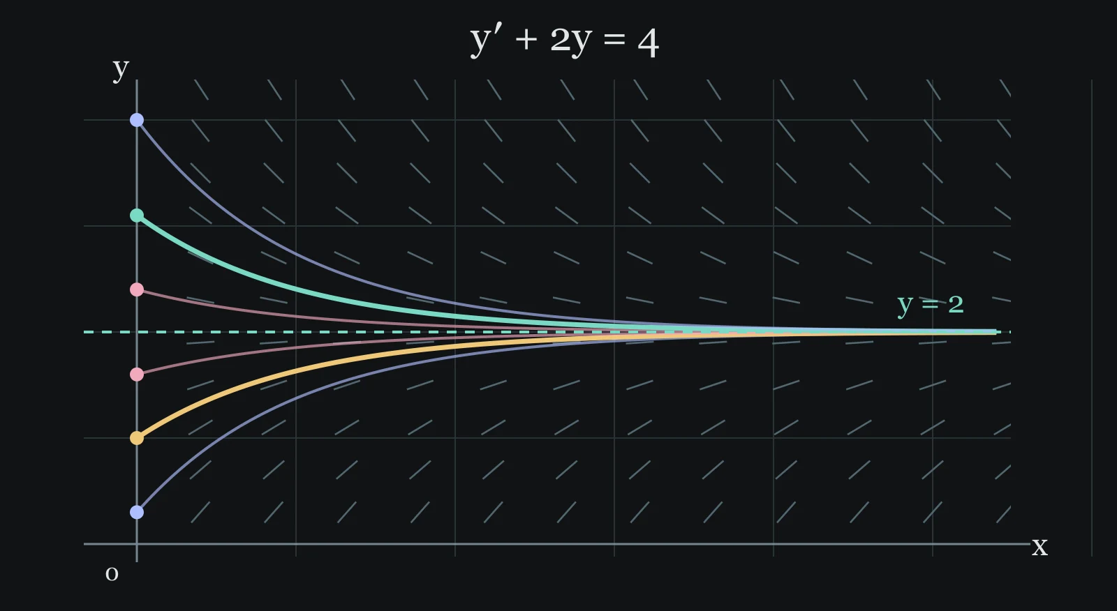
Now take $y' + 2y = 4$. As a slope rule, $y' = 4 - 2y$: below height $2$ the slope is positive, above it negative, and at $y = 2$ the graph stays level. We could separate the variables again, but we use it to learn a second method that also works when separation fails: equations of the form $y' + p(x)\,y = q(x)$, called linear first-order equations, because $y$ and $y'$ appear only to the first power.

We want a derivative we can undo. A product may help, so first work out its derivative. Write $\Delta h=h(x+\delta)-h(x)$ and $\Delta y=y(x+\delta)-y(x)$. Expanding the new product gives $(h+\Delta h)(y+\Delta y)-hy=h\Delta y+y\Delta h+\Delta h\Delta y$. Divide by $\delta\ne0$ and let $\delta$ tend to zero. The first two terms tend to $hy'$ and $h'y$. The last is $\Delta h(\Delta y/\delta)$, which tends to zero because $\Delta h\to0$ and $\Delta y/\delta\to y'$. Thus $(hy)'=hy'+h'y$. Our equation $y'+2y=4$ contains the same two kinds of term. Can a multiplier make its left side exactly this product derivative?

Multiply the whole equation by $h$: $hy' + 2hy = 4h$. For the left side to be $(hy)' = hy' + h'y$ we need $h' = 2h$. The function $h = e^{2x}$ does it, since $(e^{2x})' = e^{2x} \times 2$ by tool 3. It is never zero, so multiplying by it loses no solutions. Now follow the steps:

The third step undoes the derivative: $2e^{2x}$ has derivative $4e^{2x}$, so the two sides differ by a constant $C$. The last step divides by $e^{2x}$. With $y(0) = 1$: $1 = 2 + C$, so $C = -1$ and $y = 2 - e^{-2x}$. Check: $y' = 2e^{-2x}$ and $y' + 2y = 2e^{-2x} + 4 - 2e^{-2x} = 4$. The case $C = 0$ is the level solution $y = 2$. In the model, the left graph shows $y$ and the right graph the product $Y = e^{2x}y$: whatever the starting height, every $Y$ curve has the same slope $4e^{2x}$ at a given $x$, so they differ only by constants, exactly as the third step says.

Now let $p(x)$ and $q(x)$ be given continuous functions on the interval of interest, in the equation $y'+p(x)y=q(x)$. Matching the product rule requires $h'=ph$. Choose an antiderivative $P'=p$ and set $h=e^{P(x)}$. The chain rule gives $h'=e^P P'=ph$, exactly what we need, and $h$ is positive. This multiplier is called an integrating factor. Multiplying the equation gives $(e^Py)'=e^Pq$. Reverse differentiation and divide by the nonzero $e^P$ to obtain:

Return now to the earlier equation $y\prime=2xy$. We can check that no solution crosses zero and then leaves it. Differentiate the product $e^{-x^2}y$: its derivative is $e^{-x^2}(y\prime-2xy)=0$ by the equation. The product must be a single constant throughout the interval, including any zeros. Thus $y=Ce^{x^2}$ really is the complete family here. The product rule just derived makes this check valid even at a zero of y.

Solve $y' + \dfrac{y}{x} = x$ with $y(1) = 1$. Because $1/x$ is not defined at $0$ and our starting point has $x = 1$, we work only with $x > 0$. Here $p = 1/x$, so $P = \ln x$ and the integrating factor is $e^{\ln x} = x$. Multiplying by $x$ gives $xy' + y = x^{2}$, and the left side is $(xy)'$ by the product rule. Undo the derivative, using $(x^{3}/3)' = x^{2}$, and divide by $x$:

At $x = 1$: $1 = \tfrac{1}{3} + C$, so $C = \tfrac{2}{3}$ and $y = \dfrac{x^{2}}{3} + \dfrac{2}{3x}$. Check: $y' = \dfrac{2x}{3} - \dfrac{2}{3x^{2}}$ and $\dfrac{y}{x} = \dfrac{x}{3} + \dfrac{2}{3x^{2}}$; adding, the fractions with $x^{2}$ cancel and leave $\dfrac{2x}{3} + \dfrac{x}{3} = x$. At $x = 2$ the solution is $\tfrac{4}{3} + \tfrac{1}{3} = \tfrac{5}{3}$.

Try these

First, solve $y' = xy$ with $y(0) = -2$. Second, solve $y' + y = 3$ with $y(0) = 5$. For each, check both the equation and the starting value, then open the answer.

In the exact methods, we rearranged the equation into the derivative of an expression we could recognise, then reversed differentiation. The chain rule justified separation and the product rule justified the integrating factor. Next we will return to a solution we already know, inspect its local slopes, and ask how to construct an approximate path directly from those slopes.

We have solved and checked $y'=2xy$. Now return to the same equation with a different question: what does it tell us about the direction of a solution at one point? No new solution method is needed to read that local information.

Read it as a rule for the slope. At any point $(x, y)$ of the graph we are looking for, the slope must equal $2$ times $x$ times $y$. We can use the rule at a point without knowing the graph: at $(0.5, 1)$ the slope must be $2 \times 0.5 \times 1 = 1$; at $(1, 2)$ it must be $2 \times 1 \times 2 = 4$; anywhere on the line $x = 0$ it must be $0$. An equation like this, linking an unknown function with its derivative, is called a differential equation. Ours contains only the first derivative, so it is first order.

Move the point $P$ in the model and watch its short slope line. Then switch on the slopes at other points: the whole picture of little lines is called a slope field. A solution is a curve that is tangent to the little line at every point it passes through.

We already found $y=Ce^{x^2}$. For a chosen point $(x_0,y_0)$, substitute it: $y_0=Ce^{x_0^2}$. The exponential is positive, so division is allowed and $C=y_0e^{-x_0^2}$. Therefore the solution through that point is $y(x)=y_0e^{x^2-x_0^2}$. This is why the model can draw a whole curve after we select a point. It is using our derived solution, not guessing a curve from thirteen dots.

Notice that many curves fit the slope field, one through each starting point. To pick one, we also give a starting value, for example $y(0.5) = 1$: the curve must pass through the point $(0.5, 1)$. Such a starting value is called an initial condition. It gives a height at one $x$, not another slope.

We have an exact answer for $y'=2xy$ through $(0,1)$: $y=e^{x^2}$. Keep it as a comparison while we try another construction using only the rule. At $(0,1)$ the slope is $2\times0\times1=0$. Along that point's tangent line, a horizontal step $h=0.2$ leaves the height at 1. At the new, approximate point $(0.2,1)$ the rule gives slope $2\times0.2\times1=0.4$. A second step raises the height by $0.4\times0.2=0.08$, giving 1.08. We have replaced a changing slope over each interval by its value at the interval's start:

Take one step at a time and compare the approximate point with the exact height at the same input. This is Euler’s method, a basic numerical method. For this example and these positive steps, reducing the step gives a closer approximation over the displayed interval. That observation is not a promise for every equation or step size. More accurate numerical methods also exist. The point here is to see precisely which approximation one Euler step makes.