Artificial intelligence: from Turing’s question to large language models
Back to informaticsIn 1950 the mathematician Alan Turing began a paper with a short question: **“Can machines think?”** Seventy-odd years later, we can type a question to a program and receive a detailed, fluent answer. What happens inside such a program? Counting which words appear together gives us a small program that guesses the next word, but it remembers little context. Representing words as **lists of numbers** lets us compare them by calculation and combine information from nearby words. This leads to **attention** (letting each word use information from the others in its sentence), an important part of the **Transformer**, a structure widely used in language models. We will also examine its development and training. Generating pictures raises another question: how can a computer turn noise into an image? A method called **diffusion** will show us that process.
You do not need to know programming. We will use addition, multiplication and a few powers, and whenever a new symbol appears we will say what it means before we use it. Every number in the interactive models is actually calculated, so you can check each step yourself.
Can machines think?
Turing’s paper, “Computing Machinery and Intelligence”, appeared in the journal Mind in 1950. He noticed straight away a difficulty with his own question. To answer “Can machines think?” we would first have to agree on what “machine” and “think” mean, and people have never fully agreed about that. So he replaced it with a question that could actually be tested.
He called it the imitation game. A person, the interrogator, types questions to two players hidden in another room, one a person and one a machine, and reads their typed answers. The interrogator’s task is to decide which is which. If the machine is taken for the person about as often as a real person would be, Turing argued, we have little reason left to deny that it thinks. Today this game is usually called the Turing test.
Two further ideas in the paper matter for this page. First, Turing made a prediction. In about fifty years, he wrote, machines with enough memory would play the game well. An average interrogator would then have no more than a 70 per cent chance of identifying them correctly after five minutes of questions. Second, he suggested that instead of writing down every rule of an adult mind, we might build a machine that learns, like a child who is taught. Keep this second idea in mind, because it is exactly what modern AI does. Nobody writes the rules of a large language model; its numbers are learned from examples.
Does winning the game prove that a machine thinks? People still argue about it, and this page will not settle the question. What we can do is something more modest and more useful: understand, step by step, what today’s machines actually calculate when they answer us. Then each of us can judge Turing’s question with the mechanism in front of us rather than a mystery.
Seventy years in brief
The phrase “artificial intelligence” itself was coined a few years after Turing’s paper, for a summer workshop at Dartmouth College in 1956. Since then the field has moved between two broad ideas. The first is to write the rules ourselves: if a program should diagnose an illness, experts list the symptoms and the rules that connect them. The second is Turing’s learning machine: show the program many examples and let it adjust its own numbers until its answers agree with the examples. Choose an event on the timeline to read what happened and which of the two ideas it belongs to.
Turing proposes the imitation game and suggests building machines that learn.
A rule-based program follows steps supplied by people; a learned model uses examples to adjust its numerical settings. Both approaches have uses, and a system may combine them. More data and faster calculation helped learning methods handle larger image and language tasks. In 2017, “Attention Is All You Need” introduced the Transformer for machine translation. The small example below opens up its attention calculation so that we can check where each number comes from. Understanding how those numbers combine information will help us examine how a text generator chooses the next token. This is one important family of AI methods, not a definition of all AI.
Guessing the next word
Let us begin with the simplest version of what a language model does. Read this unfinished sentence: “The cat sat on the …”. You probably thought of “mat” or “floor”, and certainly not “idea”. You were guessing the next word, and you were guessing from experience, because you have met many sentences like this before. A language model is a program for exactly this task. Given some text, it gives a probability to every possible next word.
A probability here is a number from to that says how often we expect something to happen out of many tries. If a word comes next 1 time in 4, its probability is . The probabilities of all the possible next words add up to , because exactly one of them must come next.
The most direct way to get such numbers is to count. Below is a tiny collection of sentences, which we call the corpus, the body of text we learn from. Choose a word: the corpus marks every place it occurs, and the table lists each word that follows it there, how many times, and that count divided by the total.
| Next word | Count | Probability |
|---|---|---|
| cat | 3 | |
| dog | 3 | |
| fish | 1 | |
| mat | 1 | |
| rug | 1 | |
| Total | 9 |
For example, “the” is followed by 9 words in the corpus: “cat” 3 times, “dog” 3 times, and “fish”, “mat” and “rug” once each. So the probability of “cat” after “the” is , and the five probabilities add up to .
Now press “Write a sentence”. The program starts from your word and draws the next word at random, with each word’s chance equal to its probability in the table. Then it treats the new word as the previous word and repeats, until it reaches a full stop. This prediction, choice and append loop is an autoregressive generation method: the next choice uses the text already written. We use this method in the lesson. Other language-model tasks, such as filling a hidden word from both sides, need not generate text this way.
Counting has two serious problems. First, it knows nothing about combinations it has never seen. Our corpus never has “bone” right after “the”, so a counting model says “the cat ate the bone” is impossible, though it is a perfectly good sentence. Second, it looks only one word back. In “She lived in Paris for ten years, so she speaks fluent …”, the best next word, “French”, depends on “Paris”, eight words earlier. One word back we see only “fluent”, which says nothing about which language. We could count longer runs of words, but then almost every run is new, and nearly all the counts are zero.
We need two things. First, a way to say that words are similar, so that “bone” can borrow what we know about “fish”, since both can be eaten. Second, a way to let each word use information from anywhere earlier in the text. The next chapters build both: vectors for similarity, and attention for looking back.
In the corpus, “the” is followed by 9 words, 3 of which are “dog”. What probability does the counting model give “dog” after “the”?
Cutting text into small pieces
Before a model can calculate anything, text has to become numbers. The first step cuts the text into pieces called tokens and gives each piece its number in a fixed list, the vocabulary. Why not simply use whole words? Because the list of words never ends: names, typing mistakes, new words, numbers, other languages. Why not single letters? Because then a sentence becomes a very long sequence, and a single letter carries little meaning. Real tokenizers take a middle path: frequent words are one token each, and rarer words are built from a few frequent pieces.
9 tokens · Grey chips are single bytes (IDs 0–255).
Type into the box and watch the pieces. In “unbelievable”, our small vocabulary has no whole word, so the tokenizer takes the longest piece it knows at each point: “un”, then “believ”, then “able”. Each chip shows the piece and its ID, the token’s number in the vocabulary.
Notice what happens to a character the vocabulary does not contain at all, such as 咪 in 猫咪. It is broken into the bytes a computer uses to store it. A byte is a group of 8 binary digits, so it can take different values. Most Chinese characters are stored as three bytes. Here they are written E5, 92 and AA in base 16. Base 16 uses the digits 0 to 9 and then A to F, so every byte fits into two symbols. IDs 0 to 255 are kept for these 256 bytes, so any text at all can be turned into tokens and nothing is ever “unknown”.
Where does the vocabulary come from? It is learned from text as well. A common method, byte-pair encoding, starts from single characters and repeatedly joins the pair of neighbouring pieces that occurs most often. Step through it below on a tiny corpus of four words, each used a different number of times.
| Word | Times used | Current pieces |
|---|---|---|
| low | 5 | low |
| lower | 2 | lower |
| newest | 6 | newest |
| widest | 3 | widest |
At the first step, the pair e followed by s occurs 6 times in “newest” and 3 times in “widest”, 9 times in all. The pair s followed by t also occurs 9 times, and no pair occurs more often. When two pairs tie, the tokenizer takes the one it met first in the corpus, so “es” becomes a new piece. Then “es” followed by “t” also occurs 9 times, giving “est”. After a few merges, a common ending such as “est” and a common word such as “low” have each become single pieces, while rarer letter groups stay split. Real tokenizers keep merging until the vocabulary holds tens of thousands to a few hundred thousand pieces. As a rough guide, one English token is about three quarters of a word.
Turning a piece into numbers
Now each token has an ID. But an ID is only a name. Token 257 (“cat”) is not “close to” token 258 (“dog”) in any useful sense, and token 300 is not more of anything than token 200. We want numbers that carry meaning, so that similar words get similar numbers. The answer is to give each token not one number but a list of numbers.
A list of numbers in a fixed order is called a vector. With two numbers, say , we can draw it as an arrow from the origin of a grid to the point 3 across and 2 up. With three numbers we can draw an arrow in space. A model keeps one vector for every token in a large table, the embedding table: row 257 holds the vector for “cat”. To obtain a token’s vector, the model looks up that token’s row.
Below are 19 words, each with 8 numbers. So that you can read the numbers, I designed them by hand and gave each position a meaning. Position 1 says how much the word is an animal. Position 2 says how much it is a vehicle, and so on. Choose a word to see its 8 numbers. We can only draw three directions at a time, so the picture shows three of the eight positions. Choose which three, and drag the picture to turn it.
With the axes animal, vehicle and food, the words gather in three groups, one near each axis. Now look at the people: man, woman, king, queen, boy and girl all sit near the middle, piled on top of each other. They are not alike in every way; this particular view simply does not show the directions in which they differ. Change one axis to “person” and another to “female”, and they spread out.
This is the most important habit for thinking about vectors. A picture shows three directions at a time, but the vector has all of them. Two words can look close in one view and be far apart in the full list of numbers.
Real models work in the same way with far more numbers. The original Transformer used 512 numbers per token, and large models today use several thousand; GPT-3 used 12,288. There is one honest difference from my table: in a real model nobody chooses what each position means. The numbers start random and training (chapter 10) adjusts them. Words used in similar ways end up with similar vectors, but a single position rarely means anything as tidy as “animal”. Our labelled positions are a teaching aid that keeps the numbers readable.
How alike are two vectors?
We said that similar words should get similar vectors. How do we turn “similar” into a calculation? Start in two dimensions, where we can see everything. Take two vectors and ; the small numbers 1 and 2 only label the first and the second entry. Their dot product multiplies the matching entries and adds the results:
With more entries we do the same thing: multiply entry by entry and add everything. For example, , while , and .
Why does this measure similarity? Drag the two arrow tips below and watch the readout. When the arrows point roughly the same way, matching entries tend to have the same signs, the products are positive and the sum is large. When they are at right angles, the positive and negative products cancel and the dot product is . When one arrow is a negative multiple of the other, each nonzero matching product is negative, so their sum is negative. There is one catch: making an arrow twice as long doubles each of its entries and so doubles the dot product, although its direction has not changed.
- Dot product
- Lengths
- Cosine similarity
- Angle between them
To compare directions without including the effect of length, we need each arrow’s length. The arrow is the long side of a right triangle whose other two side lengths are and . By Pythagoras, its length is . This also equals , because . With more entries, we add their squares under the root in the same way. For nonzero vectors, dividing the dot product by both lengths gives the cosine similarity. A zero vector has no direction, so we cannot divide by its zero length. The length rule and the direction comparison are explained below:
Where does the length formula come from?
An arrow travels a units right and b units up. We need its direct start-to-end length c to distinguish direction from overall size. The horizontal and vertical sides are perpendicular, so they form a right triangle with the arrow. Start with positive a and b, and place four copies of that triangle inside the large square below.
Green shows the four triangles; gold shows the middle square. Each outer side joins lengths a and b. Every middle side is a triangle’s hypotenuse, c. Its corners are right angles because the two adjacent acute triangle angles sum to ninety degrees. One triangle has area : join it to a flipped copy to make a rectangle with sides a and b.
Now find the gold area by subtracting the four triangles from the outer square. The same area is c squared, so the two ways of counting it must agree.
A length is nonnegative, so take the nonnegative square root. For negative coordinates, use absolute coordinate values as side lengths; squaring gives the same formula. If one side is zero, the arrow is just the other side. If both are zero, its length is zero. That zero vector has no direction, and its length cannot be used as a divisor in the next comparison.
Dividing a vector by its length shrinks or stretches it to length without turning it, so this number depends only on directions. It is when the arrows point the same way, at right angles and when they point in opposite directions, whatever their lengths. The readout also shows that it equals the cosine of the angle between the arrows; the derivation below explains why, with nonzero vectors throughout.
Derivation: why the cosine similarity equals the cosine of the angle
First a fact about angles. Put two points on a circle of radius around the origin, at angles and measured from the horizontal axis. Their coordinates are and ; this is what cosine and sine mean for a point on that circle. The squared distance between them, by Pythagoras, is . Expanding and using for each point, this is .
Now turn the whole circle backwards by . The distance between the two points does not change, but now one is at angle , the point , and the other at angle . The same calculation gives a squared distance of . The two results describe the same distance, so .
Finally, write and . Then , and is the angle between the arrows. Dividing by gives the cosine of that angle. In three dimensions the two arrows lie in one flat plane through the origin and the same argument works in that plane. Beyond three dimensions we cannot draw the angle at all, so it is defined by this formula, which agrees with the drawn angle whenever we can draw it.
Now apply this to our 8-number word vectors. Choose a word in the model below: the list ranks every other word by cosine similarity calculated with all eight numbers, not only the three in the picture. “cat” and “dog” point almost the same way; “cat” and “truck” do not.
- dog
- lion
- horse
- puppy
- kitten
Vectors also allow arithmetic. Take king, subtract man and add woman: . Subtracting man removes what king shares with man, being a person and being of a certain size, and leaves mainly “royal”; adding woman then puts back “person” and the size, together with “female”. The result lies closest to queen. Learned word vectors show the same effect, but only approximately, which is why we look for the nearest word rather than an exact match.
Which pair of vectors has dot product 0?
Attention: pieces that look at each other
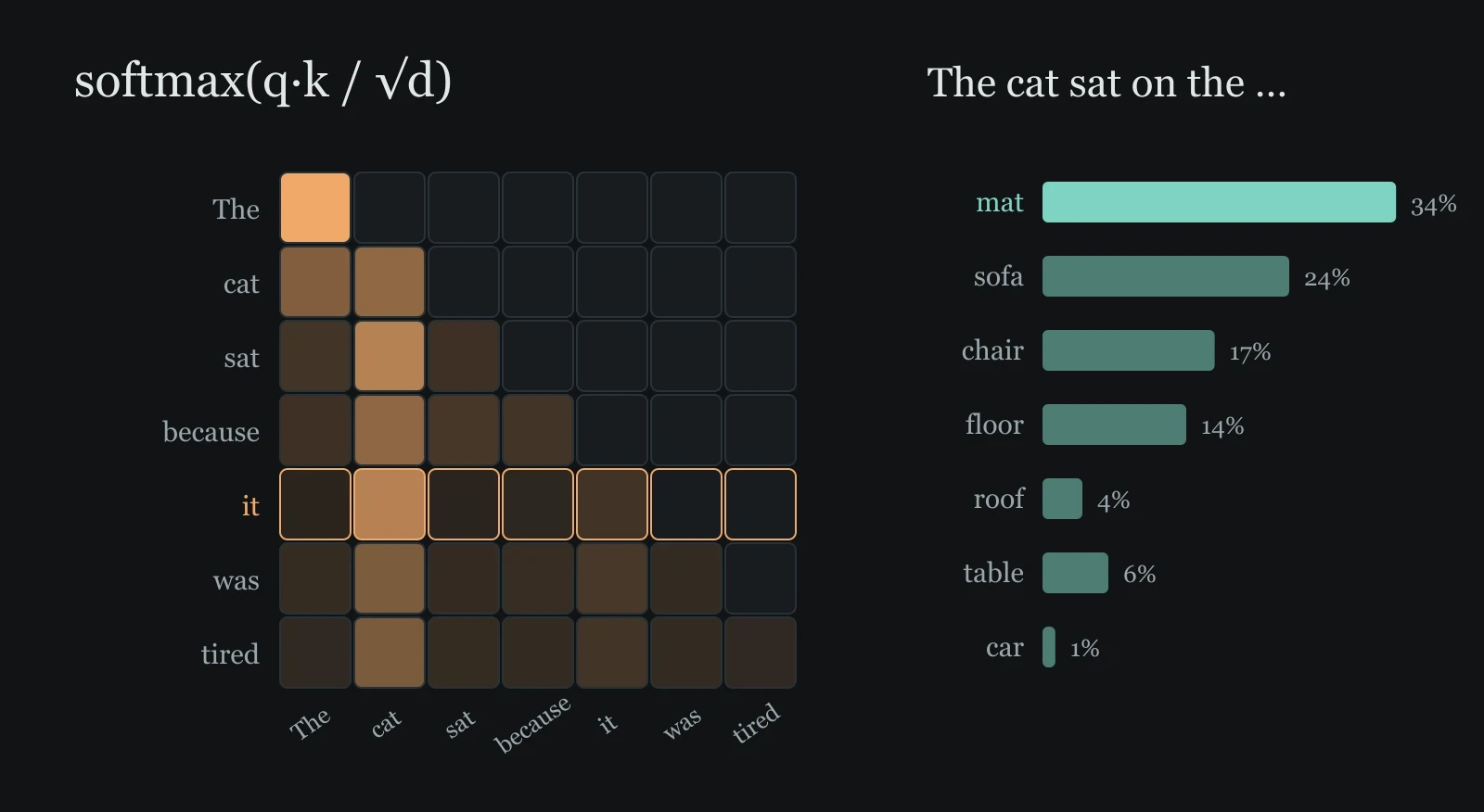
We now have a vector for every token. But the vector from the table is always the same, wherever the token appears. Look at the sentence “The cat sat because it was tired.” The table gives “it” the same vector in every sentence, yet here “it” means the cat. To understand the sentence, the vector for “it” must take in information from “cat”. In “The road was closed because it was flooded”, the same “it” would need information from “road” instead. So each token needs a way to look at the other tokens and decide which of them matter to it. This is what attention does.
Attention works like a search. Each token makes three new vectors from its own numbers:
- a **query**, which describes what this token is looking for;
- a **key**, which describes what this token offers to others who are looking;
- a **value**, the information this token passes on to whoever attends to it.
For “it”, the query says roughly “I am looking for a thing I could refer to”, and the key of “cat” says “I am a thing”. A query that matches a key well gives a large dot product, the measure of similarity from the previous chapter. So the plan is: compare the query of “it” with the key of every token it can see, and let the best matches pass on the most information.
How does a token make these vectors? In our example each token has 4 numbers, in the order [thing, pointing word, action, description]. A query and a key each have 2 numbers, so that we can draw them as arrows. To turn 4 numbers into 2, the model keeps a table of numbers called a matrix, for queries. It has one row for each of the 4 features, and each row holds 2 numbers: what that feature adds to the query. To make the query of a token, multiply each row by the token’s number for that feature, then add the four results. The numbers of “it” are , so its four rows are multiplied by , , and :
In the same way a second matrix, , makes the keys, and a third, , makes the values. The key of “cat”, whose numbers are , is : mostly “I am a thing”. Each output number is the dot product of the token’s 4 numbers with one column of the matrix, which is why this operation is called multiplying a vector by a matrix.
The score between “it” and “cat” is the dot product of the query of “it” with the key of “cat”, divided by , where is the number of entries in each query and key. We will explain the division in a moment.
Scores can be any numbers, positive or negative. We want weights instead: numbers that are positive and add up to , so that each one says what share of the attention a token receives. The softmax function turns scores into weights in two steps. Step 1: raise to the power of each score. Here is a fixed number. A power with a whole number is repeated multiplication, for example . For scores that are not whole numbers, the powers are filled in smoothly between these. A calculator gives, for example, . Two facts matter: is positive for every score , and a larger score gives a larger , so the order of the scores is kept.
Step 2: divide each result by the total of all of them. Dividing every share by the same total makes the shares add up to , just as dividing counts by their total did in chapter 3. Written with the scores of the tokens that can be seen, the weight of token is
For “it”, the tokens it may see are The, cat, sat, because and it itself, with scores , , , and . Step 1 gives about , , , and , whose total is about . Step 2: “cat” receives of the attention of “it”, and “it” itself about .
One useful property: adding the same number to every score changes no weight. Each -power becomes , so the same factor appears in every term and in the total, and it cancels in the division.
Finally, each token’s output is the weighted average of the value vectors: multiply each visible token’s value by its weight and add them up. For “it”, of the result comes from the value of “cat”, so the new vector of “it” carries mostly the information of “cat”. In the model, the value arrows are laid tip to tail, each shrunk by its weight, and the last tip is the output.
One more rule. When a model writes text, a token may look only at itself and the tokens before it, because the later ones have not been written yet. Their scores are left out; we can think of them as a score of , whose -power is . This is called a causal mask. Switch it off in the model to see what an encoder, which reads a whole finished text at once, would do.
Choose the token that looks. The left picture shows its query (gold) and the keys of the tokens it can see (grey). The bars show the scores and the softmax weights. The right picture lays the weighted values tip to tail to make the output (gold). The grid below holds every token’s weights at once: row = the token looking, column = the token looked at.
Why divide by ? A dot product adds up products. In a real model each query and key has 64 or 128 numbers, and adding many products tends to give large scores. Large differences between scores make softmax put nearly all the weight on one token. Then learning stalls. A token with weight close to hardly affects the result, so it hardly receives any correction (chapter 10). Suppose the entries behave like random numbers of typical size . Then the dot product of of them has a typical size of about . Dividing by brings the scores back to a typical size of about . Switch the division off in the model: the weight of “cat” for “it” rises from to , and the other weights shrink.
Derivation: why the typical size of a dot product is
Let the dot product be , where every entry is an independent random number with average and average square . To measure the typical size of we look at the average of , then take its square root.
Expanding gives squared terms and many cross terms with . Each squared term averages to , because and are independent. Each cross term contains, for example, , which is independent of everything else in that term and averages to , so the whole cross term averages to .
So the average of is , and the typical size of is . Dividing by makes the average square of the score , whatever is. Learned queries and keys are not exactly such random numbers, so this is a guide for choosing the scale, not an exact law.
One head forms one weighted combination of values at each position. Its role need not be one fixed, human-readable relationship. A Transformer runs several heads side by side, each with its own three matrices, and joins their outputs. Switch to Head B: with different matrices, the same tokens now look for the most recent action rather than the thing being referred to. The original Transformer used 8 heads in each layer, and large models use dozens. Nobody tells a head what to look for; like the word vectors, its matrices are learned, and only some heads turn out to have a tidy meaning.
If every attention score in a row is increased by , what happens to the softmax weights?
Building a Transformer
Attention lets tokens exchange information. A Transformer layer surrounds it with a few simpler steps, and the whole model is a stack of identical layers, each with its own learned numbers. Choose each part of the diagram to see what it does and why it is there.
Several heads (chapter 7) let each token gather information from the tokens it can see.
Follow one normalisation, entry by entry
After addition, entries may share a large offset or be widely spread. Removing their common offset centres them around zero. Adjusting their spread changes how far apart they are. We use just two entries below, and each step keeps earlier results so we can trace every new value. For now, the final learned scale is 1 and the offset is 0.
A real layer may then multiply entries by learned scales and add learned offsets. After that, the mean and variance need not be zero and one. We have unpacked this operation’s arithmetic, not claimed that normalisation guarantees successful learning.
Why are positions needed? Attention combines tokens through dot products and weighted averages, and neither of these cares where a token stands. If we shuffle the sentence, the outputs are just shuffled in the same way. In the demonstration below both sentences contain the words dog, bites and man, and we run Head A from chapter 7 over all three tokens, with no mask. Compare the output for “dog” in the two sentences.
Without positions the two outputs are exactly equal, so the model could not tell who bit whom. With a position vector added to each token, one fixed pattern for each place in the sentence, the outputs differ, and later layers can use the difference.
The original paper built its position vectors from sine and cosine waves of different lengths. Many models today instead turn each query and key by an angle that depends on the token’s position (rotary position embedding), so that a dot product depends on how far apart two tokens are.
In the 2017 paper the Transformer was built for translation, for example from English into German. It had two halves. The encoder read the whole English sentence at once, with no mask. The decoder wrote the German sentence one token at a time, with a causal mask. In each layer it also attended to the encoder’s output, in order to see the English sentence. This is called cross-attention. The base model had 6 layers in each half, 512 numbers per token, 8 heads and about 65 million learned numbers, and it trained in about 12 hours on 8 GPUs. Its larger version set new records for English–German and English–French translation. The GPT family of language models keeps only the decoder half, without cross-attention: it reads the text so far and writes the next token.
Optional: the one-line formula in the paper
The paper writes chapter 7 in a single line, . Here is a table whose rows are the queries of all the tokens, and and are the tables of keys and values. , read “ transposed”, is with its rows turned into columns.
Multiplying the table by the table produces, in row and column , the dot product of query with key : all the scores at once. Softmax is applied to each row, giving the grid of weights in our model. Multiplying that grid by forms, for each row, the weighted sum of the values: all the outputs at once. Nothing new happens in this line; it is our calculation for every token together, which is exactly what a GPU does fastest.
Choosing the next piece
Let us return to “The cat sat on the …”. After the last layer the model holds one vector for the last token. To score each candidate next token it takes the dot product of with that token’s vector: a large score means points the way the candidate does. These raw scores are called logits. In our toy, vectors have 4 numbers for [something to sit on, indoors, soft, food], , and “mat” has the vector . So the logit of “mat” is .
Softmax, the same function attention used, turns the logits into probabilities. Then the model must choose. Always taking the most likely token sounds sensible, but it makes text repetitive and dull, and every answer to the same question identical. So models usually sample: they draw a token at random, each token’s chance being its probability. Press “Draw one” a few times, then “Draw 100”, and compare how often each word was drawn with its probability.
The cat sat on the ____
0 draws. Green bars: probability. Thin gold bars: share actually drawn.
The temperature divides every logit before softmax. With nothing changes. To see what does, compare two candidates with logits and . The ratio of their probabilities is , because the total in softmax is the same for both and cancels, and this equals . For “mat” and “sofa”, with logits and , the ratio is at and at . So a temperature below stretches the differences and favours the likely tokens even more; as approaches the model almost always takes the top token. A temperature above shrinks the differences, and unusual words appear more often.
Two more controls cut off the long tail of unlikely tokens before drawing. Top- keeps only the most likely tokens. Top- keeps the most likely tokens until their probabilities add up to at least , so it keeps few tokens when the model is confident and more when it is unsure. In both cases the kept probabilities are divided by their new total, so that they add up to again.
Having drawn a token, the model appends it to the text and runs again to choose the next one: exactly the loop of the counting model in chapter 3, only with much better probabilities. A long answer is thousands of these steps, and each step is a full pass through every layer.
With a temperature very close to , what does sampling do?
Where do the numbers come from?
All the numbers we have met, the embedding table, the matrices of every head and the feed-forward matrices, are called parameters. GPT-3 has 175 billion of them. Where do their values come from? They start as small random numbers, and training adjusts them with a very simple task. Take real text, hide the next token, and let the model predict it. Then nudge every parameter so that the correct token would have been a little more likely.
To nudge in the right direction we need one number that says how wrong the prediction was. If the model gave the correct token probability , we use the loss . Here is the natural logarithm, which undoes raising to a power: is the power to which must be raised to give . When the loss is ; when it is about ; when it is about . The loss is small when the model was confidently right and grows without limit as the correct token’s probability approaches .
Why a logarithm? The probability the model gives a whole text is the product of the probabilities of its tokens, one after another. The logarithm of a product is the sum of the logarithms. Write and . Then , so . Therefore the loss of a whole text is simply the sum of the losses of its tokens, and each token can be treated as its own small example.
Now the nudge. For each parameter, calculus gives its slope: how fast the loss changes when that parameter increases by a tiny amount, which is its derivative. For a differentiable loss with a nonzero gradient, a sufficiently small step against that gradient lowers the loss locally; an arbitrarily large step has no such guarantee. This is called gradient descent, and the size of the step is set by the learning rate (eta). To see the arithmetic, our small experiment adjusts the three output logits themselves, not every internal parameter. For these logits the slope has a remarkably simple form: for the correct token it is , and for every other token it is that token’s probability . Writing for the correct token and for the others, one step is
So a step raises the correct token’s logit by and lowers each wrong token’s logit by . Step the training below; the correct answer is “mat”. At the start the logits are , and , so and the loss is about . After one step with , the logit of mat rises by to , while sofa and moon fall by their probabilities, and . Each step makes the correct answer more likely, by less and less as approaches . A larger learning rate moves faster, but in a real model with billions of parameters too large a step overshoots and the loss jumps about, so the rate is chosen with care.
| Next word | Logit | change | ||
|---|---|---|---|---|
| mat · correct answer | 0.50 | −0.68 | +0.68 | |
| sofa | 0.80 | 0.44 | −0.44 | |
| moon | 0.20 | 0.24 | −0.24 |
- Step
- 0 / 12
- Loss
Derivation: where the slope comes from
Write the logits as and the total of their -powers as . If token is correct, , so the loss is . We used and .
Now change one logit . The term changes at rate if and at rate otherwise, which is . For we use the chain rule: the derivative of is , and changes at rate when changes, because the derivative of is . So changes at rate . Adding the two parts, the slope of the loss with respect to is .
Earlier parameters affect the final loss through intermediate calculations. Backpropagation reuses the chain rule to combine these local rates efficiently; it is not a separate source of correct answers. The small example below multiplies two local rates so we can see why an earlier parameter receives its change. Next-token prediction is one training objective. Instruction examples, preference feedback and other objectives can be added later, so we should not infer that everything an assistant does came only from this one objective.
How does an earlier parameter receive a change?
Use a chain we can calculate completely: the input is 2, the parameter is w and the prediction is . We want 3. Call the error , and square it to obtain the loss , so positive and negative errors cannot cancel. Change only w and follow its effect through to the loss.
If w increases by h, the error increases by 2h. Substitute that into the square, subtract using ordinary algebra, then divide by h. Only then let h approach zero. This gives the slope we need here.
We can also split the chain: the error changes twice as fast as w. The square’s local rate with respect to the error is 2a, because . Multiplying the two rates gives . Backpropagation combines such local relationships in order; this short chain makes the multiplication visible.
η is the step size you choose. Try 0.1, then reset the weight and try 0.3. Both move against the slope, but the larger step overshoots and increases the loss. A sufficiently small step depends on the function; an arbitrary step is not guaranteed to work. The minimum is at , where the error is exactly zero. The readout rounds to three decimal places, so it uses ≈ for approximate equality. Each update still uses unrounded values; treating the displayed approximations as exact inputs can give a different final digit.
Where the Transformer came from
Before 2017 the standard tool for language was the recurrent neural network, or RNN. It reads a sentence one token at a time, like a person reading with a finger under the line, and carries a single memory vector forward. At each step it combines the memory with the new token’s vector to make the next memory. After the last token, the memory is supposed to hold the whole sentence.
This design has two weaknesses. Information from an early token must survive every later step before it can be used at the end, and it fades along the way, much like a message passed along a line of people. The LSTM (1997) added gates, learned switches that decide what to keep, what to forget and what to add, which helped the memory last longer but did not remove the problem. The second weakness is speed. Step 50 needs the memory from step 49, so the steps cannot be calculated at the same time, while GPUs are fastest when they do thousands of calculations at once.
In 2014, translation systems called sequence-to-sequence models used one RNN to read the English sentence into a memory vector and a second RNN to write the French sentence from it. Squeezing a whole sentence into one vector was a bottleneck, and long sentences came out badly. The same year Bahdanau, Cho and Bengio let the writing RNN look back, at every step, at all of the reading RNN’s memories, with weights calculated from how well each memory matched what it needed. That was attention, added as a helper to an RNN.
The Transformer’s authors asked what would happen if attention did all the work and the step-by-step memory were removed altogether. That is the meaning of the title “Attention Is All You Need”. Every token can reach every earlier token in a single step, and, when the entire training sequence is already supplied, many positions can be calculated in parallel while the mask hides later answers. During ordinary autoregressive generation, the next token still depends on the token just chosen, so those new choices occur sequentially. Compare the two designs below: choose the length of the text and see how many steps information from the first token needs to reach the last.
- Steps from first to last token
- Steps that must happen one after another
- Comparisons per head
- —
Attention is not free. With the causal mask, token number compares itself with tokens, so a text of tokens needs comparisons in each head of each layer.
To add this up, write the sum twice, once forwards and once backwards, and add the two lines term by term: , , and so on, each pair making . There are pairs, so twice the sum is , and the sum is . For 1,000 tokens that is comparisons, and doubling the length roughly quadruples the work. This is why long texts are expensive, and why much later research went into making attention cheaper. The time complexity lesson explains this kind of growth.
From the Transformer to today’s large models
Within a year, two uses of the Transformer appeared. GPT (OpenAI, 2018) kept the decoder and learned to predict the next token using a large collection of books. This is called pre-training. Further training on small labelled sets for particular tasks is called fine-tuning. BERT (Google, 2018) kept the encoder and learned to fill in hidden words using text on both sides, which suited tasks such as search and classification. Both showed that training on large amounts of raw text could learn language patterns useful for several tasks.
Then came growth. GPT-2 (2019) had 1.5 billion parameters; GPT-3 (2020) had 175 billion and was trained on about 300 billion tokens. GPT-3 showed something new: without any further training, it could do a task after seeing a few examples written into the prompt, such as a few English–French pairs followed by a new English sentence. In 2020 researchers measured that the loss falls smoothly and predictably as parameters, data and computation grow together; these are called scaling laws. In 2022 the Chinchilla study found that many models were too large for the amount of text they had seen. A good balance is roughly 20 training tokens per parameter. Chinchilla had 70 billion parameters and was trained on tokens, that is 1.4 trillion.
The chart shows published sizes. Each grid line up the side is ten times the one below it. We need such a scale because the sizes range from 65 million to 671 billion, about four steps of ten, and on an ordinary scale every model before 2020 would be squashed flat against the bottom. Choose a point to read its details. Several of the strongest models never published their size, so they are not shown rather than guessed.
GPT-3 · 2020 · Parameters: 175 billion
A model trained only to continue text is not yet an assistant: asked a question, it might reply with more questions. Two further stages of training turned it into one. In instruction tuning, the model is trained on examples of requests together with good responses written by people. In reinforcement learning from human feedback (RLHF), people compare pairs of the model’s answers. A second model learns to predict which answer people prefer. The language model is then adjusted to give answers that this second model scores highly. InstructGPT (2022) showed that people preferred the answers of a model trained this way with 1.3 billion parameters to those of the original 175-billion-parameter GPT-3. ChatGPT, released in November 2022, brought the result to the public. Anthropic, the company that trains Claude, introduced a related method, Constitutional AI, in which the model also critiques and revises its own answers against a written list of principles.
Since then the basic machine has remained the Transformer, while many of its parts have been improved.
The feed-forward step is split into many smaller networks, the experts, and a small router sends each token to only a few of them. The model can hold a great many parameters while each token uses only some: DeepSeek-V3 (2024) has 671 billion parameters but uses 37 billion for each token.
The amount of text a model can attend to has grown from 2,048 tokens for GPT-3 to hundreds of thousands. Some models now reach a million or more. Cheaper ways of computing attention and better ways of encoding position made this possible.
Pictures, sound and video are cut into small patches and turned into vectors, so the same attention can mix them with words.
Since 2024 some models are trained, by reinforcement learning on problems whose answers can be checked, to write out long chains of intermediate steps before answering. This greatly improves their results in mathematics and programming.
Models are trained to call search engines, run code and operate software, so that they can carry out tasks of many steps.
The best-known families today include GPT (OpenAI), Claude (Anthropic), Gemini (Google), Llama (Meta), DeepSeek and Qwen (Alibaba). Some publish their parameters for anyone to download; others do not publish even their size.
It is worth being clear about what has not changed. A model still produces one token at a time from probabilities learned from its training text. It can state false things fluently, which is called hallucination, because a likely continuation is not always a true one. Its knowledge stops at its training data unless it is given tools such as search. And how far its calculations amount to “thinking” is exactly Turing’s question, which is still open.
Diffusion: drawing by removing noise
We have followed a text generator that chooses one token after another. Next we study a different method for generating images: diffusion. First we need to know what a picture is to a computer: a grid of pixels, each holding a number for its brightness (three numbers, for red, green and blue, in a colour picture). A small grey picture is just numbers.
Now add noise. To every pixel add a random number drawn from the bell-shaped normal distribution, where most draws are close to and a few are larger. Do it gradually over many steps, while multiplying the original brightness numbers by a smaller factor, without changing the image dimensions, and the picture fades into pure noise. After step the pixels are
Here is the original picture, (epsilon) is the noise, and (read “alpha bar t”) is the share of the original that survives: it starts at and falls to almost . So the picture is a mixture of two ingredients, the original weighted by and the noise weighted by . Move the slider to add noise; the readout follows one pixel through the formula. Why square roots? Their squares add up to exactly : . This choice keeps variance equal to 1 only under a stated model: the clean-data variable and independent noise both have variance 1. It does not mean that the visible contrast of every fixed photograph stays unchanged. For a fixed clean pixel, only the noise is random, with variance 1 minus alpha-bar. The derivation below separates these cases and explains why squares appear.
- share surviving
- One pixel:
Adding noise is easy and needs no learning. The clever part is running it backwards. We train a neural network on millions of pictures with a simple task: given a noisy picture and the step , guess the noise that was added. This task is easy to set up, because we made the noisy picture ourselves and know the right answer. Once the network can guess the noise, we can also guess the clean picture by rearranging the formula above:
The little hats mean “estimated”. To get this, subtract from both sides of the forward formula, which leaves on the right, then divide both sides by .
To make a new picture, start from pure noise and walk the steps backwards. At each step, guess the clean picture and work out the noise that this guess implies. Then put the two back together at the next, slightly lower noise level. Use the forward formula with in place of . Early on the guesses are vague averages; as the noise falls they sharpen, and at the last step , so the result is the final guess itself. This version of the walk is called DDIM; the original method, DDPM, also adds a little fresh noise at each step.
A whole picture has too many numbers to draw as one point, so the model below uses the smallest possible “pictures”: single points with numbers. The training data are 240 points along a heart. On the left tab, add noise and watch the heart dissolve into a round cloud. On the right tab, generate: 500 points of pure noise walk back onto the heart. Choose one point to follow its path and the guess made at each step.
- share surviving
Our small model does not need a trained network because it knows all 240 training points. Its guess of the clean point is a weighted average of these points. As in attention, softmax turns scores into weights. A training point receives a score for how well it explains the noisy point . How do we calculate that score? The forward process shrinks to , which is where this clean point would be before noise was added. The squared distance from to that position measures their difference: a shorter distance gives a better match. Dividing by twice the noise share, , and adding a minus sign makes shorter distances give higher scores:
Why divide by the noise share? Early in generation the noise share is large, so even far-off training points get scores close to the best one; many points share the weight and the guess is a blurry average. Near the end the noise share is tiny, the nearest point wins almost all the weight, and the guess becomes sharp. This is the same softmax-weighted average as in attention, with the noisy point as the query and the training points as both keys and values. The optional note derives the score.
Derivation: why the squares count, and where the toy’s scores come from
The spread of a random number is measured by its variance: the average of its squared distance from its average. Take , where and are independent with average . The average of is . Independence and average make the average of equal to , so the variance of is . With pixel values scaled to variance and noise of variance , the weights and give variance at every step.
Now the scores. If the clean point was , then , so the noise must have been . We assume independent standard-normal noise coordinates. Their probability density is proportional to , where the squared length sums the squared noise coordinates. Density describes the relative chance of landing in equally small neighbourhoods, not a positive probability at one exact real number. Substituting the required noise gives a likelihood proportional to , which is raised to the score.
Before seeing , every training point was equally likely. By Bayes’ rule, the probability that came from is then its likelihood divided by the total of all the likelihoods: exactly softmax of the scores. The guess with the smallest average squared error is the average of the possible clean points weighted by these probabilities, which is the formula the toy uses.
Why average the possible clean points?
The point model above begins by treating each stored clean point as equally likely. For the current noisy observation, a clean point receives more weight if its noise model gives that observation greater density. The shared prior probability and Gaussian density constant cancel between numerator and denominator, leaving each exponential score divided by their sum.
Those weights do not yet tell us which number to output. We must state the objective: which guess minimises average squared error? Start with one coordinate. The candidate clean values are , their weights are , their weighted mean is , and our guess is u.
Split the difference from guess to candidate into guess-to-mean and mean-to-candidate. After expanding the square, the cross term vanishes: the definition of the mean makes the weighted deviations sum to zero.
The second term on the right does not change with u. The first is a nonnegative square, equal to zero at . Therefore the weighted mean is the best guess under squared error. In two dimensions, add the two coordinate errors and apply the same reasoning to each. This generally differs from choosing the single most probable point: the result depends on our stated squared-error objective.
Our toy explicitly stores a finite set of 240 clean points and computes its estimate from them. As its noise level becomes very small, its weights concentrate near those stored points, so its output tends towards this finite set. A real diffusion model instead learns a function from examples; that function can generalise to new combinations, but it can also memorise or reproduce training material. A finite network size does not rule out memorisation. Our small point experiment demonstrates its chosen empirical distribution, not a guarantee of originality or an account of every image model.
How does a prompt such as “a cat on a mat, oil painting” steer the picture? The text is first turned into vectors by a Transformer. At every step the denoising network attends to those vectors through cross-attention, as in the translation Transformer. So its guesses are pulled towards pictures that match the words. To save work, Stable Diffusion (2022) runs the whole process on a compressed version of the picture rather than on every pixel. This is called latent diffusion. Many newer image and video models use a Transformer as the denoising network itself. So the two halves of this page meet: attention and diffusion now work together.
In the forward process, what is at the very start, ?
Back to Turing’s question
Let us return to Turing. In 1950 he suggested a test based only on conversation, and a machine that learns rather than one programmed rule by rule. Today’s language models are learning machines of exactly that kind. They hold a table of vectors, attention that lets tokens consult one another, and small networks inside each token. Billions of parameters are adjusted so they predict the next token of an enormous amount of text.
Whether that amounts to thinking is still debated. In the simplified generator we studied, each next-token choice is calculated from learned numbers and the supplied context. A complete assistant may also use written instructions, retrieval and other programmed tools. Understanding the learned calculation helps us check its facts, distinguish fluent wording from reliable evidence, and ask more useful questions.