Electromagnetic induction: from circuits to generators
A bicycle dynamo can light a lamp while the wheel turns. There is a wire, a magnet and some movement, but no battery supplying the lamp. Where does the electrical energy come from, and why does the lamp go out when the wheel stops? We will build up an answer by following the apparatus and the energy, beginning with an ordinary battery circuit.
We will first separate two questions: how much charge passes through a wire each second, and how much energy is supplied to each portion of charge. Then we remove the battery and examine what moving a magnet can do. You will see the wire, the loop and the meter stay easy to follow as we connect the physical parts to the graphs. You can pause, move the time slider and repeat an observation.
01 Start with a wire and a battery
Look at the battery, switch and resistor on the bench below. The leads join them into a route that can be closed or broken. The wire already contains charged particles: a metal contains electrons, and some can move through it. The battery does not manufacture a new batch of electrons or wait for one electron to travel all the way to the resistor before it works. Closing the route establishes an electrical influence along the circuit, called an electric field; the mobile charges respond to it.
Charge is a property that determines how a particle participates in electrical interactions. There are positive and negative charges. An electron has negative charge. We measure an amount of charge with the coulomb, abbreviated C, and use the symbol for that amount. A coulomb contains the charge magnitude of a very large number of electrons; the markers in our drawings represent portions of charge, not individual electrons drawn to scale.
Choose a cross-section of the wire, as if we had drawn a counting line across it. If an amount passes in a time interval , the average current is the amount per unit time. This is the definition of average current, not a new experimental law. The symbol means “change” or “interval”. One ampere, A, means one coulomb passing per second.
We conventionally point current in the direction positive charge would move. Mobile electrons in a metal drift in the opposite direction because they are negative. We will use conventional current consistently, including every direction arrow below.
Current tells us how much charge passes. We also need to know how much energy can be transferred per unit charge. A battery providing for each provides : voltage is measured in volts, V. A joule, J, is a unit of energy. Write transferred energy as and charge as . Energy delivered per charge and charge delivered per second answer different questions.
A resistor transfers electrical energy into thermal energy. For the simple resistor we use here, measurements give a current proportional to its voltage when temperature stays fixed. Its resistance is the ratio and is measured in ohms, . Rearranging gives , then . This behaviour is called Ohm’s law; not every electrical device follows it.
Follow the complete path
The battery is on the left, the switch is at the back, and the resistor is at the front. Close the switch to complete the circuit and press play. Orange markers follow the wire in the conventional current direction. Each represents an amount of charge, not an individual electron. The marked cross-section counts charge passing through it: the amount equals current multiplied by elapsed time.
- Battery
- Switch
- Resistor
- Charge-counting section
Drag to inspect the apparatus, or use the view buttons. The lesson controls also change this view.
The switch leaves a visible gap. The battery still supplies a voltage, but there is no sustained current. Close the switch before starting this charge-counting experiment.
- Resistance
- Current while the circuit is connected
- Charge counted over the selected interval
- Energy transferred to the resistor
The playback control freezes our observation clock; it is not another electrical switch. Opening the actual switch breaks the path. For the selected interval, multiply the amount of charge by energy per charge to find the energy transferred: W = VQ. Keep these two ratios separate: current is charge per second; voltage is energy per charge.
We have now separated the charge already present, the energy supplied per charge and the current through a complete path. Keep that distinction. Next we ask whether a battery is the only way to supply this electrical driving action. We will need to describe a magnet before we can test that question.
02 How we describe a magnetic field
A magnet can affect another magnet without touching it. To describe the influence at different locations, we assign a magnetic field to each location. A field is a way of recording a local physical condition: which direction it points and how strong it is there. The arrows are our representation of that condition; they are not little material rods filling the space.
A small compass helps assign direction. Its north-seeking end points along the local field. Outside a bar magnet, field arrows leave its north pole and enter its south pole; the pattern continues through the magnet as closed field lines. We use for magnetic field magnitude and tesla, T, for its unit. When we say a field is uniform, we mean it has the same direction and magnitude throughout the region under discussion.
A field line is a drawing aid. Drawing twice as many lines on the same diagram does not physically double the field. We show field strength through an explicit numerical value; line density or darkness is only a visual guide. This matters because we are about to measure how a field passes through a chosen surface, and literal counting of a few drawn lines would give a misleading answer.
Electric current also produces a magnetic field. A current around a loop makes a field through its interior. A coil is a wire wound into several loops, called turns. Therefore a coil can respond to an external magnetic field and also create a field of its own. We will keep those two fields distinct when we determine the direction of induction.
03 One surface, a chosen direction, and flux
The copper loop below has an open middle. Turn on “Opening surface”: a translucent sheet fills exactly the opening bounded by that same wire. This is a drawing aid we have added, not a membrane in the apparatus. Turn it off and the wire remains unchanged. Why add it? We want to compare how a magnetic field passes through the whole opening, so we need to identify the area we are comparing.
Start with a uniform field passing straight through the sheet. For this perpendicular crossing, we define magnetic flux as field strength multiplied by area . Doubling the area doubles the amount of surface exposed to the same field. Doubling field strength doubles the flux through the same area. Flux is measured in webers, Wb.
Now rotate the copper frame. Its translucent opening surface turns with it. The blue field arrows keep their direction. The green arrow stays perpendicular to the surface; we call this a normal. It provides a definite direction to compare with the field, even when the face turns edge-on. There are two opposite normals; we choose one and keep tracking it. The angle between this chosen normal and the field is called theta, written .
We can obtain the crossing area by projecting the sheet onto a plane perpendicular to the field. For a rectangular sheet rotated about one edge, that edge keeps its length . Its other edge, length , projects to . Here cosine is the signed projection ratio: in a right triangle it is adjacent side divided by hypotenuse. Thus the original area is , while the signed projected area is . We label this signed projected area . Multiply that crossing area by the uniform field to obtain the flux.
Keep track of the same surface
The copper frame encloses the opening surface we use to measure flux. Blue arrows show the applied field; green marks the chosen normal, perpendicular to the surface. Show the translucent sheet and its projection onto the fixed screen on the right. Orange guides run parallel to the field, joining each corner of the frame to the matching corner of its projection. Looking “Along the field” lets you check that they line up.
- Copper frame
Drag to inspect the apparatus, or use the view buttons. The lesson controls also change this view.
Compare the copper frame with the translucent projection. Rotating changes the area facing the field. Increasing the frame area enlarges both the actual calculation surface and its projection; it is not only a change in the readout.
- Actual loop area
- Projected area magnitude
- Signed flux through the chosen surface
The filled face, projection, normal and field arrows are explanatory overlays. The physical apparatus contains the copper frame and magnetic poles, not a membrane or solid arrows. The apparatus is enlarged for inspection; the stated area is the one used in the calculation.
When the normal points with the field, and : flux is . When the field lies in the surface, and the projected crossing area is zero. When the normal points against the field, and flux is . We have not lost the field; the minus sign preserves its direction relative to our choice.
For a field that varies across a surface, one product is not enough. Divide the surface into small patches. On each patch use its local field, area and normal, then add the signed contributions. The integral symbol is compact notation for the limit of these finer sums. Our experiments use a flat loop and a uniform field where the simple product is exact.
The index labels a patch; is its area. In the integral, names the surface, is a tiny area contribution and is its unit normal, an arrow of length one specifying direction. The dot between the vectors means take the field component along that normal. No new physical law has been added here: this extends our definition of flux.
04 From a changing flux to an emf
We can now describe the magnetic situation through the loop. But that still leaves the question that started the lesson: can this arrangement drive charge without a battery? Compare the instrument while the field is held steady and while the field is changing. Before calculating its response, let us recall what the battery supplied: energy for each amount of charge, rather than new charge.
Suppose a source can supply 0.08 joule for each coulomb taken around a circuit. Dividing energy by charge gives 0.08 joule per coulomb, or 0.08 volt. This energy-per-charge driving quantity is called electromotive force, shortened to emf and written . The historical name contains “force”, but this is not a mechanical force measured in newtons. With a battery, chemical processes supply the energy; with induction, a changing magnetic field can provide the electrical driving action. A conducting path is still needed for a sustained current.
For a stationary loop, induced emf is the work the induced electric field would do per unit positive charge taken once around the loop. This is a whole-loop quantity. In a changing field it cannot in general be replaced by one path-independent voltage between two points. An open circuit can therefore have induced emf without a sustained current.
Faraday’s experiments established the connection we need: changing the magnetic flux through a circuit produces an emf around it. This is an experimental physical law. We will calculate its consequences, but the definition of flux and a drawing of field arrows alone cannot prove the law.
Let be the flux at the beginning and the flux at the end. Their change is final minus initial, . Dividing by the elapsed time gives the average rate of change. For a coil with identical turns connected in series, each turn contributes the same emf, so the contributions add. Faraday’s law then gives the average emf shown below. We will interpret its minus sign in the next direction experiment.
Suppose one turn’s flux increases from to in . Subtract first: the change is . Divide by time: each second contributes an average increase of . Twenty series turns multiply the emf by twenty. Therefore its magnitude is . This is an average; if the change is uniform, it is also the emf throughout the changing interval.
Watch where each point on the graph comes from
Keep the copper loop fixed between the field poles. Blue arrows describe a uniform applied field that we control. Play to increase or decrease that field over the selected time. The moving point below records the same instant: its horizontal coordinate is elapsed time, and its height is the flux through one turn. The switch changes the conducting path, while the imposed field programme stays the same.
- Chosen calculation surface
Drag to inspect the apparatus, or use the view buttons. The lesson controls also change this view.
The current meter spans −0.02 A to +0.02 A. Opening the switch returns this needle to zero, even while a changing flux still produces emf.
The apparatus shows one representative turn. The calculation uses N identical series turns, each enclosing the same area. The applied field programme is an ideal controlled input; the arrows do not claim that this pole shape was solved as a precise field simulation.
- Applied field now
- Flux now, per turn
- Live emf
- Live current
- Average for the complete selected change
The field is being held at its present value, so the live emf is zero. The average comparison refers to the complete change you selected, not to this stationary moment. Play again to make the field change.
Keep the two endpoint fields unchanged and double the time. The graph reaches the same height in twice the horizontal distance; the average rate, and hence the emf magnitude, halves. We neglect the winding’s own induction here. Abrupt starts and stops are idealisations; the later self-induction experiment explains why real circuits respond more gradually.
If the flux changes unevenly, the whole-interval average hides when the change was fastest. Take a smaller time interval around the moment of interest and calculate the same quotient. When these quotients approach a definite value as the interval shrinks, that value is the instantaneous rate, written . We do not put zero in a denominator; we take a limit of nonzero intervals.
For example, suppose a prescribed changing field gives , with and time measured in seconds. We can find its rate without skipping the algebra. Expanding the square gives ; subtracting the original cancels that term. Dividing by the nonzero interval leaves . The last term tends to zero, so the rate is . The formula describes a chosen input, not a claim that every real magnet follows a square law.
At , the instantaneous rate is . With twenty turns, the instantaneous emf is . Between two and three seconds, however, the average rate is , giving . The two answers differ because the flux is changing faster as time increases.
05 Why a nearby magnet is not enough
Return to an ordinary magnet beside a coil. The magnet’s field at the coil becomes stronger as it approaches, so the flux changes. If we stop the magnet, a magnetic field is still present, but that field is no longer changing. The distinction is between having flux and changing flux. A large constant flux can give zero emf, while a smaller but rapidly changing flux can give a substantial emf.
Move in, hold still, and withdraw
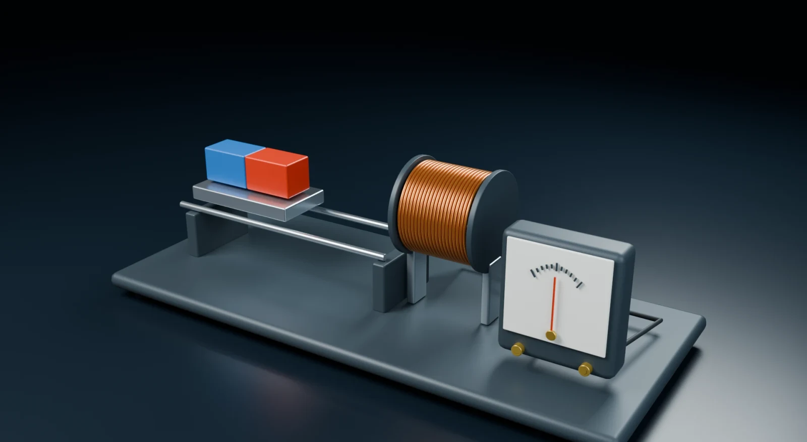
The coil stays fixed while the magnet moves into its hollow centre. Play the approach, hold the magnet still, and withdraw it to compare these three situations. You can pause anywhere to inspect the apparatus or drag the position control while paused. The live meter returns to zero when the magnet is still. The separate comparison below keeps the average over the whole journey; that average does not mean a current is still flowing now.
- Copper winding
- Bar magnet
- Zero-centre meter
Drag to inspect the apparatus, or use the view buttons. The lesson controls also change this view.
The meter reads current on a −0.02 A to +0.02 A scale. A moving magnet can still produce emf when the switch is open, but this broken path cannot carry a sustained current.
- Flux through one turn now
- Live emf
- Live current
- Average over the selected endpoints
The hole is real geometry: the magnet enters between the copper turns without passing through a solid wall. Its changing flux is represented by a smooth teaching profile, not measured data from this rendered magnet. The live emf is calculated from the slope of that same profile multiplied by the actual motion speed. A slower journey gives a smaller response; holding any position gives zero emf. The positive flux direction is to the right along the coil axis.
Movement by itself is also insufficient. If a rigid closed loop translates entirely inside a uniform, steady field without rotating or changing area, its flux stays constant and its net induced emf is zero. Individual wire segments may have magnetic forces on their charges, but their contributions around the whole loop cancel. Moving into or out of a field region changes the area exposed to the field, so that is a different situation.
Likewise, we can leave every wire still and change the field using another coil whose current changes. Faraday’s law asks us to track the flux, not to search for a moving object at all costs. The three factors in show three routes in the uniform-field case: change field strength, exposed area, or orientation.
06 Work out the direction with Lenz’s law
The magnitude calculation does not yet tell us which way current would flow. A current makes its own magnetic field, so its direction matters. Lenz’s law states that the induced emf acts in the direction whose current would oppose the change in flux. The word “change” carries the whole distinction: when the original flux is decreasing, the induced field helps maintain its original direction.
Decide what changes before choosing a current direction
Use the same hollow coil, with rightward along its axis chosen as positive. Choose the direction of the applied field and whether its strength is growing or shrinking. Blue arrows show that applied field. The orange arrow revealed by the second decision shows the field produced by the induced current. Both fields occupy the same space, but they come from different sources.
- Copper winding
- Zero-centre meter
Drag to inspect the apparatus, or use the view buttons. The lesson controls also change this view.
The applied flux points right. Its magnitude is increasing.
To oppose an increase, the induced field points against the applied field.
Look from the right end of the coil. A current that runs counterclockwise as seen from that end makes a rightward field; clockwise makes a leftward field. This is the measured current-loop rule, represented by the moving orange markers.
The field is being held still. There is no continuing induced current during this hold. Play to observe the direction you have just worked out.
We can now read Faraday’s minus sign. Choose the normal toward yourself and pair it with counterclockwise positive circulation, using the right-hand rule. If outward flux increases, is positive and circulation is clockwise. If outward flux decreases, is negative, the emf becomes positive and circulation is counterclockwise. Changing our sign convention changes both labels, not the physical prediction.
Why is this opposition sensible? Suppose pushing a magnet into a closed resistive coil induced a current that helped the magnet move farther in. Motion would make more current; that current would accelerate the magnet; the resistor would also heat. This proposed self-amplifying process would create energy without a source. The observed opposing response instead makes the person pushing the magnet do work. Conservation of energy is a consistency check on the direction; the measured induction law supplies the quantitative relation.
Opposing a change does not mean perfectly cancelling it. Resistance, geometry and self-inductance determine how large the current becomes. A resistive coil usually cannot keep the original flux exactly unchanged. We will see the energy balance explicitly with a sliding rod.
07 What pushes the charge?
So far we have a reliable loop rule, but it is reasonable to ask what actually acts on the charge. There are two useful situations. A stationary wire in a changing magnetic field experiences an induced electric field. A wire moving through a magnetic field carries charges that experience magnetic forces. Both can contribute to the emf, and a real apparatus may contain both.
For the first situation, the electric field can circulate around a region of changing magnetic flux. It exists even if no wire is put there; a wire provides mobile charges with a conducting route. This is different from the electrostatic field of fixed charges, where the total work per charge around a closed path is zero. The changing-field case is precisely where that closed-path total can be nonzero.
For the moving-wire situation, use the experimentally established magnetic force law. A positive charge moving with speed perpendicular to a field experiences magnetic force magnitude , perpendicular to both motion and field, given by the right-hand rule. The symbol refers to the charge we are following; it need not be a whole coulomb. An electric field exerts force on the same positive charge. Below, labels magnetic force and labels electric force.
First imagine an isolated metal rod, with its length , velocity and magnetic field mutually perpendicular. Magnetic forces redistribute the mobile electrons toward one end, leaving a positive charge imbalance at the other; the positive metal ions remain bound in the lattice. This charge separation builds an electric field in the rod. It grows until its electric force balances the magnetic separation force, giving the balancing field .
Why does this give a voltage? A constant electric force acting over distance does work of magnitude . Divide work by charge to obtain the potential difference magnitude . Therefore the open rod has an end-to-end potential difference . In a rail circuit, the moving rod contributes the motional emf ; the complete circuit and its resistance then determine current.
Move one side of a complete circuit
The copper rod rests across two conducting rails. The resistor joins the rails on the left, making a closed circuit. Blue arrows point down through the horizontal loop. Moving the rod to the right enlarges the area; reversing it shrinks the area. Play one journey and watch the shaded swept strip grow with the same position shown on the ruler. Pausing holds the rod still, so the live emf and drag become zero.
- Sliding rod
- Resistor
Drag to inspect the apparatus, or use the view buttons. The lesson controls also change this view.
- Displacement from the left position
- Live emf
- Live current
- Required pull magnitude
- Mechanical input / resistor heating
The physical rod length used here is 0.4 m and the illustrated journey is 0.8 m. A top view puts the downward field into the screen, matching the direction convention in the derivation. Reversing motion reverses emf and current, while heating remains positive. We neglect friction, rail resistance and self-inductance. The magnetic field enables the transfer; the person or machine pulling the rod supplies the energy.
Now verify the same magnitude from flux. During a short time , a rod moving at constant speed advances a distance . The new rectangular strip has width and height , so its area is . Multiply by the perpendicular uniform field to find . Dividing by time cancels the nonzero and gives again. The local magnetic-force account and the loop-flux account agree.
In the diagram, motion is rightward and the applied field points into the screen. The positive magnetic force in the rod is upward, so current goes up the rod and counterclockwise around the loop. That current creates an outward field, opposing the increasing inward flux. We obtain the same direction by both methods.
08 Where the electrical energy comes from
An emf does not tell us that energy is free. Close the rod circuit and it carries a current. The applied field then exerts a force on the current-carrying rod, opposite its motion. To keep the speed constant, an external pull must balance that magnetic drag. We will derive the amount rather than merely attach an energy label to the animation.
To find the force on the current, suppose the rod contains mobile positive charge carriers per unit volume, each of charge , drifting along the rod at speed . Let the wire’s cross-sectional area be . During time , carriers in a length cross a counting plane. Their number is , their charge is , and dividing by time gives current . This is a convenient equivalent positive-carrier model; using negative electrons gives the same conventional-current result.
A length of rod contains such carriers. Each has a magnetic force magnitude associated with its drift along the rod. Add these forces: . Group the factors as the current just obtained, giving magnetic drag force opposing motion.
Mechanical work from a steady pull over a distance is . Divide by the time taken and use to obtain mechanical power . Electrical energy transferred to charge is ; divide by time and use to obtain electrical power . Power means energy transferred per second and is measured in watts, W.
Finally, for our resistive load , so its heating power is . This proves the equality of input mechanical power and output heating in the ideal steady model. The energy comes from the person or machine pulling the rod, while the magnetic field enables the transfer.
There is a subtle point: a magnetic force is perpendicular to a charge’s total instantaneous velocity, so that force alone does no work on a point charge. In the moving conductor, charge separation, electric fields and the external mechanical constraint act together. It would therefore be misleading to describe the static magnetic field as a fuel that is consumed to power the resistor.
09 Turn the motion into a generator
A sliding rod cannot keep moving along a finite rail forever. A rotating coil solves the practical problem: it can return to its starting position and repeat. Its area and the external field stay constant, but the angle changes continuously, so its flux changes. A generator converts the mechanical work needed to maintain that rotation into electrical energy.
Angular speed tells us how quickly an angle changes. To define a radian, take a circular arc of length on radius and set its angle to . Therefore when the angle is in radians. Divide by time for uniform rotation: the speed of a point at radius is . Starting face-on, the angle at time is , and the previously derived flux rule gives flux .
We can find the emf without assuming you know the derivative of cosine. Take a rectangular coil rotating about an axis through its centre, parallel to its two long sides. Call each long side’s length and its distance from the axis . Their separation is , so the enclosed area is . Each long side moves at speed .
When the normal is aligned with the field, each long side is moving parallel to the field at that instant, so no magnetic separation force acts along it. As the coil turns by , the side’s velocity turns through that angle relative to the field. Its component perpendicular to the field has magnitude : sine is the perpendicular projection ratio, opposite side divided by hypotenuse in a right triangle. This is the component that enters the rod result.
Each long side contributes emf magnitude . The two sides move oppositely, but they are also traversed in opposite directions when we go around the loop, so their loop contributions add. The short sides contribute no emf along themselves for this geometry. Two long sides and series turns therefore give . Replace by , and use the sign convention consistent with decreasing positive flux at the start: the signed result is .
One continuous turn, two connected measurements
The copper rotor turns between fixed magnetic poles. Its chosen normal turns with it. The two graphs use the same angle: blue is flux per turn and orange is induced emf. Start face-on, then inspect a quarter turn before playing a full turn. Playback is deliberately slowed to one quarter of the selected physical speed; the speed used in the calculation is shown explicitly.
Drag to inspect the apparatus, or use the view buttons. The lesson controls also change this view.
The model has one open copper turn connected through insulated slip rings, fixed brushes and a load. The calculation represents twenty identical series turns. This is an apparatus construction view, not a claim that the one visible turn is physically twenty turns.
- Flux per turn now
- Live emf
- Peak at the selected running speed
The rotor is held still, so its live emf is zero. The orange curve remains as a comparison: it gives the emf at each angle if the rotor were turning at the selected physical speed.
The maximum magnitude of sine is one, so the peak emf is . More turns, a larger area, a stronger field or faster rotation can each increase it within the assumptions of this model. A half-turn reverses the sign of the emf. With a resistive load this gives a current that reverses periodically: alternating current, AC. Maintaining the rotation under load requires mechanical work; the generator is not an energy source independent of its drive.
10 Two coils and a transformer
We can also transfer energy between two separate coils. Drive an alternating current through the first coil, called the primary. Its changing magnetic field links a second coil, called the secondary, and induces an emf there. The charges in the primary wire do not have to jump into the secondary wire. Energy is transferred through the electromagnetic field.
For an ideal transformer, assume every turn of both windings links the same changing core flux, and ignore winding resistance, magnetic losses and leakage flux. Let the primary have turns and the secondary turns. Each turn has the same flux rate. Faraday’s law therefore gives and . Dividing their nonzero amplitudes cancels the shared rate, giving voltage ratio equal to turns ratio: .
The symbols and here represent effective AC voltages. “Effective” means a constant voltage that produces the same average heating in a resistor. Since the entire secondary waveform is the primary waveform multiplied by the same turn ratio, its effective value is multiplied by that ratio too. Coil winding direction also determines relative polarity; the displayed ratio compares magnitudes.
Doubling secondary voltage does not double available power for free. In a lossless transformer with a resistive load, average input and output powers are equal: . Divide by the nonzero product to get . Thus a voltage increase is accompanied by an inverse current relation. Changing the load changes how much power the source must provide.
Follow the same changing field through both windings
The two windings share a core but have no electrical connection to each other. Follow the coloured field markers around the core while the primary supply alternates. The second meter follows the changing shared flux. Changing the secondary turn count changes its voltage; the apparatus uses representative visible wraps, and the exact turn count is written beside the controls.
Drag to inspect the apparatus, or use the view buttons. The lesson controls also change this view.
Each visible wrap represents ten turns. The primary has ten visible wraps, representing 100 turns. The secondary changes by one visible wrap for each ten-turn step. The green arrows show a direction around the core; they are a field overlay, not material travelling through the iron.
- Primary turns
- Selected secondary RMS voltage
- Live secondary voltage
- Average load power during alternation
The effective values describe a complete running cycle. They are comparisons, not the instantaneous held-state voltage. The live readout is zero when the field is held still. A larger secondary voltage draws the corresponding input power from the primary source; the transformer does not multiply energy.
A steady current produces a steady core flux, so it cannot maintain secondary induction after the switching transient. This is why an ordinary transformer needs a changing input. Electronic power supplies may begin with a DC source and switch it rapidly, creating the changing current the transformer requires. Real devices also lose energy as heat and can saturate their cores, so the ideal ratios describe a useful limit, not a promise of lossless hardware.
11 A coil can induce an emf in itself
Until now, we often treated the induced current as emf divided immediately by resistance. But a coil’s own current makes magnetic flux. If its current changes, that self-produced flux changes too, inducing another emf in the same winding. This is self-induction. It explains why a coil can resist a change in current without preventing current itself.
Add the flux linked by all turns and call the result flux linkage . For identical turns, . In a fixed coil whose materials respond linearly, linkage is proportional to its current. We define the proportionality constant as inductance : . This proportionality is a model for that coil and operating range, not a universal rule for every magnetic material. Applying Faraday to the linkage and holding constant gives the self-induced emf.
Inductance is measured in henries, H. Rearranging the emf relation shows : an inductance of one henry corresponds to an emf magnitude of one volt when current changes by one ampere per second. Rising positive current gives a negative self-induced emf; falling positive current gives a positive emf. It opposes the change, exactly as Lenz’s law required.
Where does the extra work done against self-induction go? In an ideal inductor it is stored in the magnetic field. We can calculate it using small increments of current. To increase current, the source must overcome a voltage . In a short interval , charge passes. The small energy supplied is voltage times charge, so . The time factors cancel; the energy depends on how far the current is increased.
To add these contributions from zero current to a final current , plot vertically against horizontally. Because is constant, the plot is a straight line from the origin to height . Each small energy is a narrow area under that line. All the areas together form a right triangle: half the rectangle with base and height . Therefore the stored energy is . The factor one-half comes from building the field gradually; using final voltage or final current for every earlier increment would overcount.
Change the coil’s own current
Begin with a steady current of one ampere in the same coil. Choose a final current and the time for the change, then play. The green field grows or shrinks with the current; the orange indication is the emf opposing that change. During a pause the imposed current is held fixed, so the live self-induced emf is zero even though magnetic energy remains stored.
- Copper winding
Drag to inspect the apparatus, or use the view buttons. The lesson controls also change this view.
This view isolates the winding and its field. The supply that sets the current is outside the view; the orange numerical instrument below reports the self-induced emf.
- Current now
- Live self-induced emf
- Magnetic energy now
- Mean emf for the selected change
Increasing current requires additional work from the source; the magnetic energy rises. The opposing emf acts against the increase. When we hold the current steady, that opposing emf vanishes but the stored energy remains.
Here an ideal external controller prescribes the current. The coil remains linear with L = 0.5 H. The instrument indicates the self-induced driving quantity, not the total voltage supplied by that controller. A practical switch-on curve also depends on the resistance and source, which this comparison holds outside the model.
When current decreases, the coil can return this stored energy to the circuit. Trying to stop current very quickly makes large, so the required voltage can be large. This is why practical circuits include paths or components that manage switching transients. The lesson’s steady resistor approximation is useful when self-induction has a negligible effect on the timescale being studied; it is not the full response of every real coil.
12 Use the chain of reasoning yourself
For each problem, keep the same order: identify the loop and choose its normal; find which part of the flux changes; calculate final minus initial and divide by time for an average; determine direction with Lenz’s law; calculate current if a circuit model is specified; and identify the energy source.
A coil has fifty turns, each enclosing an area of . Its normal points with a uniform field that increases from to in . Find the average emf and the average current in a closed purely resistive loop.
Show the reasoning
The angle is zero, so each turn has flux . Compute both endpoints before multiplying by the number of turns. Positive circulation is paired with the stated normal.
The negative signs mean circulation opposite to the chosen positive direction. The induced field opposes the increase of the applied flux. The source changing the external field supplies the energy.
Hold a strong magnet still beside a fixed coil. The coil has a large magnetic flux. Must it have a large induced emf? What changes if we withdraw the magnet?
Show the reasoning
No. While everything is stationary, the flux is constant, so and . Withdrawing the magnet changes the flux. The induced current, if the circuit is closed, makes a field that helps maintain the disappearing flux, and the magnetic response resists the withdrawal.
A perpendicular rod of length moves at through a field. The completed circuit has resistance . Find emf, current, drag force and mechanical input power.
Show the reasoning
The equality checks the energy transfer. A larger pulling force would accelerate the rod unless some additional opposing force were present; these values describe constant speed with the stated idealisations.
An ideal transformer has two hundred primary turns and fifty secondary turns. Its primary effective voltage is , and the secondary is connected to a resistor. Find both currents. Then explain why a steady primary current would not maintain the same secondary voltage.
Show the reasoning
The current ratio is inverse to the voltage ratio. After a steady primary current is established, its flux stops changing, so the secondary emf becomes zero. The turn ratio alone cannot create induction without changing shared flux.
A linear inductor of carries . Its current then falls uniformly to in . Find its mean self-induced emf and the energy released from its field.
Show the reasoning
The positive emf is along the original positive current direction, opposing its decrease. The released energy goes into the rest of the circuit according to the available path; the inductor does not create that energy at switch-off.
Sources and the status of the model
The laws used here are experimentally established electromagnetic laws. The geometrical, algebraic and energy consequences are derived within the lesson. The drawings and numerical examples were constructed for this lesson; they are not measurements of a particular generator or magnet. The following sources were checked for the physical laws and their limits.
- Feynman Lectures, II–17: The Laws of Induction — local force and flux accounts
- OpenStax, University Physics II, 13.1 — flux and Faraday’s law
- OpenStax, 13.2 — Lenz’s law
- OpenStax, 13.3 — motional emf
- OpenStax, 13.6 — generators
- OpenStax, 15.6 — ideal transformers
- OpenStax, 14.2 / 14.3 — self-induction and field energy