Biology · molecules to evidence
How can DNA samples be compared?
Suppose two labelled tubes contain material collected from different places. Both may contain human cells, and both may contain DNA. Looking at the tubes will not tell us whether the DNA came from the same person. We need a property we can measure, and we need to understand exactly what a matching measurement would mean.
We will follow one small example from cells, through selected DNA regions and copying, to visible bands. The laboratory equipment can be inspected in three dimensions. Alongside it, slower diagrams show the molecular reasoning that real equipment hides inside a tube. All profiles and frequency numbers below are invented for teaching.
A sample is not a visible fingerprint
A cell is a small unit of living tissue. Many of our cells contain a nucleus, a compartment surrounded by a membrane. The nucleus contains chromosomes. Each chromosome is a long DNA molecule with proteins that pack it up. Those proteins are not what this lesson compares; we compare the order of bases along the DNA. A molecule is a group of atoms joined by chemical bonds. DNA is a very large molecule built from linked units called nucleotides. A strand is one chain of those units. Their bases come in four kinds, abbreviated A, T, C and G. A sequence is the order of those bases along a strand. Keep three words as you read on: DNA, base, sequence.
Most human DNA sequence is shared between people. We therefore do not look for a completely different molecule in each person. Instead, we choose several locations where a small measurable difference can occur. The resulting collection of measurements is a DNA profile. “DNA fingerprint” is a name for this comparison; it is not a photograph of a fingerprint-shaped molecule.
The first station below shows the collection context. Select a station, then use Next step. This bench keeps the equipment in a stable view; it will not spin or jump while you read. We will return to what happens inside the tubes in the next sections.
1/3 · A labelled tube
We keep a label with the sample throughout the process. A correct measurement of the wrong person’s sample would still give a wrong conclusion.
Drag to inspect the apparatus. The camera never rotates by itself. Use “View from above” for the gel, or reset a view after turning. These are teaching models, not instructions for handling biological evidence.
What can differ between two people?
Consider a short sequence, GATA. At a selected position, it may occur directly beside another copy: GATA GATA GATA. There are three repeats here. A different copy of that chromosome can have more or fewer repeats at the corresponding position. A short sequence repeated side by side is called a short tandem repeat, abbreviated STR. The location we compare is called a locus.
For the ordinary chromosome pairs used in this example, a person has one copy inherited from each biological parent. Therefore we read two repeat counts at each locus, such as 8 and 11. A particular version at that locus is an allele. Here, “allele 8” means the version with eight repeats; it is not the eighth chromosome and not eight copies of the entire DNA molecule.
Keep these three things separate: the locus is the location; the repeat count describes a version found there; the two counts together describe this person at that location. The repeat need not be part of a protein-making gene. Our A, B and C are invented locus names, not the DNA letters A and C being counted.
Turn repeat counts into lengths
DNA normally has two complementary strands: A pairs with T, and C with G. One matched pair is a base pair, abbreviated bp. Thus a double-stranded region with 132 paired positions is 132 bp long, even though it contains 264 individual bases across the two strands. We measure length along the molecule, not by adding both strand lengths.
We copy the repeating region together with fixed sections on its two sides. For our fictional locus A, those fixed sections total 100 bp. Every GATA repeat contributes four more base pairs. With eight repeats, the repeated part is , so the complete copied piece is . With eleven, it is .
Keep the ends fixed; change only the repeats
Each red GATA block represents four base pairs. The two grey ends together represent 100 base pairs. They are compressed on the screen, so compare the numbers, not the drawn widths.
- Copy 1 length
- Copy 2 length
- Different lengths
- 2
The copies have different lengths. Their amplified fragments form two groups, so we expect two bands at this locus in the ideal clean sample.
Let be the number of repeats and the measured length. The same counting gives . To find how many repeats are present, we need the length of the repeating part. Removing the fixed 100 bp gives . Each repeat occupies four bp, so dividing the remaining length by four gives . For a measured 152 bp piece, bp belong to the repeats, and , so this piece has thirteen repeats in our model.
A and B can both have eight repeats without producing the same fragment length: our fictional B includes 160 fixed base pairs, so its eight-repeat fragment is . We must keep the locus label. Real alleles can also have partial repeats or other sequence differences; our whole-repeat arithmetic deliberately leaves those cases out.
From cells to a usable extract
Before copying any region, we need to release DNA from the collected material. A prepared solution opens the cell membrane and nuclear membrane. Proteins and other substances can interfere with the copying reaction, so extraction includes removing them and collecting DNA in a suitable liquid. The exact steps depend on the sample and the method; opening a cell is only the first part.
Select Release DNA on the bench. The large rotor is the part of the centrifuge that spins the tubes. We keep it still so you can inspect where the tubes sit. Rotating can help separate material, but the instrument does not read a DNA sequence. A labelled tube keeps the extract connected to the original sample; separate tools and controls help detect contamination.
An extraction control that contains no collected sample is carried through the process. A later DNA signal in that control can indicate contamination. Measuring a clean negative control is therefore part of understanding a result, even though it produces no exciting band pattern. This lesson shows ideal clean samples; real laboratories must check quantity and quality before interpretation.
Choose the region before copying
The extract contains DNA from many locations, but we only want the chosen STR regions. There may also be too little of them for a clear measurement. We therefore make many copies of the selected regions, using a method called the polymerase chain reaction, or PCR. The selection must happen as part of copying; multiplying every unrelated piece would not answer our particular question.
Proteins are another kind of large biological molecule. Some help chemical reactions occur; these are called enzymes. A DNA polymerase is one such enzyme. Here it joins new nucleotides into a strand by following a template. A single template base fixes the complementary base to add: template A calls for T, T for A, C for G, and G for C. But the enzyme needs an existing short strand to extend. We supply this starting piece as a primer.
The two ends of a DNA strand are chemically different, named and . DNA polymerase adds to the end, so the newly made strand grows in the to direction. We do not need the sugar’s atom numbering to follow the diagram; we do need to keep the two ends distinct. A primer is a short starter that lies against the template; the enzyme adds to its free end. The two templates point in opposite directions, which is why the primers below must face opposite ways.
Why do we need two primers?
Read the two long grey lines as the original strands. The small paired marks represent bases; this is a direction diagram, not a molecular shape. Gold sections are the primers and teal sections are DNA built from them.
The original strands point in opposite chemical directions. and name their two chemically different ends; they do not give a distance or an angle. The pairing is complementary: A pairs with , and with .
The pair of primers attaches to matching sequences on opposite sides of the chosen region. In later cycles, copies made from earlier copies acquire both primer-defined boundaries. Why the third cycle? Follow the three steps below: the first fixes one end, the second fixes the other, and only the third gives a product with both strands at the target length. Exact-length double-stranded products first appear by the end of the third cycle in the ideal model starting from one longer double-stranded molecule. Heating does not cut the chosen segment out of a chromosome; repeated copying creates the bounded pieces.
Why cycling makes many copies
Return to Copy a region on the bench. Heating separates the strands; cooling allows primers to attach; a suitable warmer temperature lets the enzyme extend them. The instrument repeats these stages. In our illustration they are about 95 °C, 58 °C and 72 °C, but the correct settings depend on the actual primers, enzyme and protocol. A temperature is not a universal instruction for every PCR.
An ideal doubling model
We start with one already bounded, double-stranded target fragment. Each ideal cycle copies both strands fully: one double strand becomes two double strands. Keep that starting assumption in mind as you change the cycle count.
Every pair of lines is one whole double-stranded copy. After one cycle: . After two: . Repeating that multiplication times gives . This is a count of fragments, not of individual strands.
This ideal doubling calculation explains why repeated copying can produce a strong signal from a small start. It does not mean a real reaction doubles perfectly forever. Reagents become limiting, the enzyme can lose activity, and copying efficiency changes; the reaction eventually approaches a plateau. Also, the first cycles from a long chromosome contain products with different boundaries. The simple count above deliberately starts from an already bounded target fragment.
Make the lengths separate
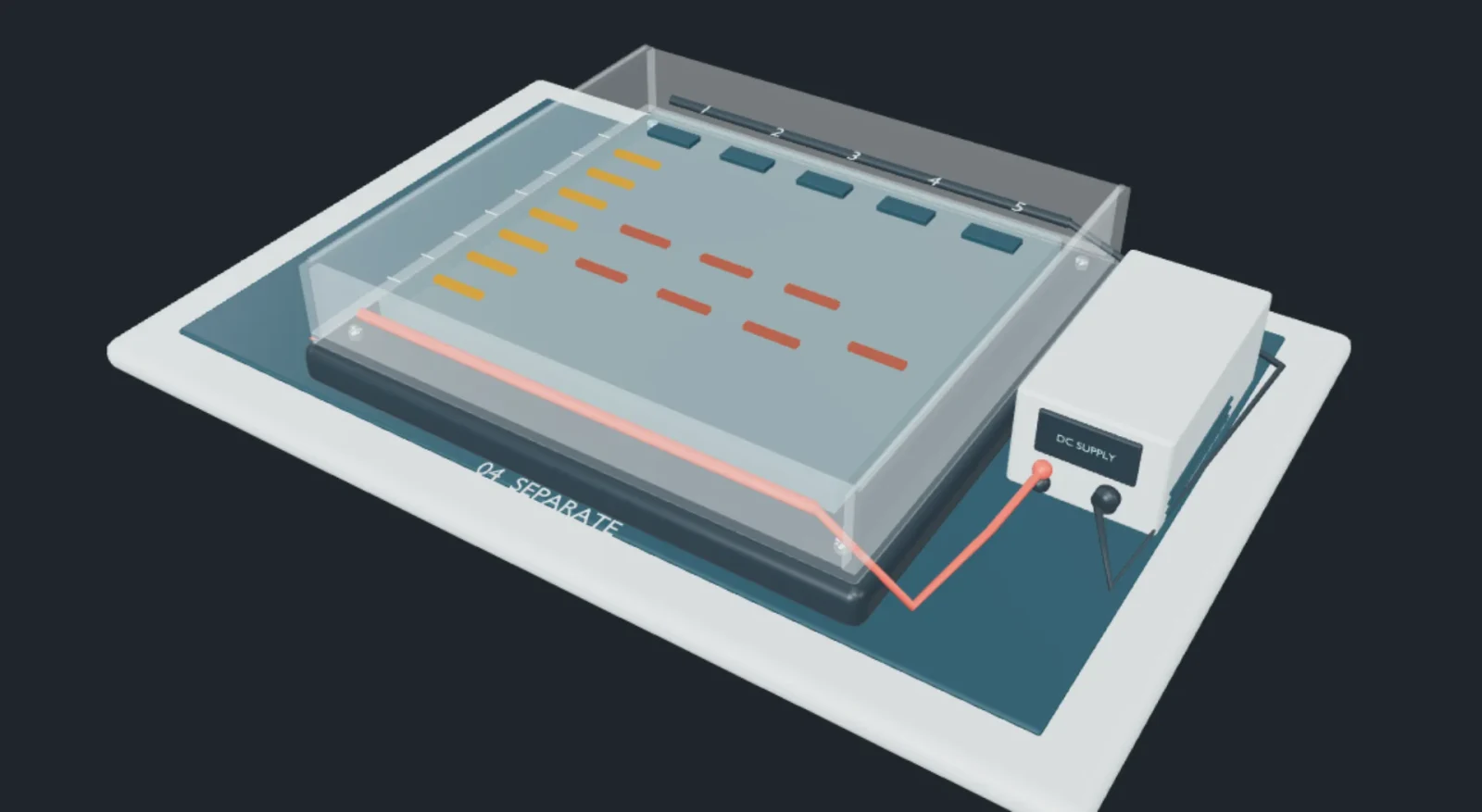
Now we have many copies, but we still need to measure their lengths. DNA’s backbone carries negative electrical charge under the usual conditions of this separation. Electric charge is a property that determines electrical forces; opposite signs attract. A voltage between two electrodes establishes an electric field; electrodes are the conducting contacts connected to the power supply. The field drives negative DNA towards the positive electrode. This gives a direction, but direction alone does not sort lengths.
For separation we add a porous material: a gel. It contains a network with small passages. For the same type of DNA under suitable conditions, shorter fragments pass through more readily and migrate farther in a fixed time. This observed size separation is the physical starting fact of the model. The screen’s evenly readable spacing is a teaching choice, not a formula for a particular gel.
The wells hold the samples at the starting end. Each well begins one lane, so a lane is a sample’s path through the gel. Many fragments of equal length collect into a visible band after detection. A known collection of lengths in a separate lane acts as a ruler, called a DNA ladder. A band below a longer reference band has travelled farther and corresponds to a shorter fragment.
Select Separate lengths on the bench and choose View from above. Press Run separation, pause, or drag the progress control. Change only the selected locus and watch the same labelled lanes. At A, 132 bp is shorter than 144 bp, so it travels farther; the corresponding repeat counts are eight and eleven. The numerical comparison below makes the result readable even without precise dragging.
Compare without losing the labels
We now compare a fictional unknown sample with three reference samples. A reference is material known to come from a particular person. Here all samples contain DNA from one person, all measurements are correct, and every allele is detected. Under those assumptions, a different pair at even one locus means the profiles do not match. Matching only A is not enough; inspect B and C too.
Read one locus, then check the next
The wells are at the top, beside −. DNA travels down towards +. The numbers beside lane 1 are known fragment lengths in base pairs. Match a sample band’s height to this reference, then read the table.
The real gel is transparent until a detection method makes DNA visible. This bright display represents detection, not naturally glowing DNA. Each locus is shown separately, with enlarged separation.
| Lane / sample | Repeat counts | Fragment lengths |
|---|---|---|
| 1 · Reference | 4, 6, 8, 10, 12, 14, 16 | Known lengths |
| 2 · Unknown | 8 / 11 | 132 / 144 bp |
| 3 · Person 1 | 8 / 11 | 132 / 144 bp |
| 4 · Person 2 | 8 / 11 | 132 / 144 bp |
| 5 · Person 3 | 9 / 9 | 136 / 136 bp |
Person 1 shares A’s and C’s . At , Person 1 is , while the unknown sample is . Person 2 shares all three pairs. Person 3 differs at all three. This is why we retain both numbers and their location instead of counting how many bands look roughly similar. Two different loci are different questions.
How inheritance constrains the pairs
The same kind of profile can check whether inheritance is compatible with a proposed family. For each ordinary chromosome pair in this example, a child receives one copy from each parent. We assume no new mutation and no measurement error. At , the child has , while the mother has . The shared 10 can come from the mother; she has no 12, so the other parent must supply 12.
Repeat the reasoning at : the child is and the mother , leaving 9 for the other parent. At : the child is and the mother , leaving 9. The required numbers in this particular example are therefore 12 at , 9 at and 9 at . If both child values occur in a parent, the origin may be ambiguous; we must check both assignments rather than always “subtracting the first number”.
Read one locus, then check the next
The wells are at the top, beside −. DNA travels down towards +. The numbers beside lane 1 are known fragment lengths in base pairs. Match a sample band’s height to this reference, then read the table.
The real gel is transparent until a detection method makes DNA visible. This bright display represents detection, not naturally glowing DNA. Each locus is shown separately, with enlarged separation.
| Lane / sample | Repeat counts | Fragment lengths |
|---|---|---|
| 1 · Reference | 4, 6, 8, 10, 12, 14, 16 | Known lengths |
| 2 · Mother | 7 / 10 | 128 / 140 bp |
| 3 · Child | 10 / 12 | 140 / 148 bp |
| 4 · Adult A | 8 / 11 | 132 / 144 bp |
| 5 · Adult B | 12 / 13 | 148 / 152 bp |
Adult A lacks 12 at A, so the example is incompatible there. Adult B carries all three required numbers, so this simple check does not exclude that adult. It does not establish a biological relationship. Actual parentage analysis uses additional loci, population information and explicit statistical hypotheses, while considering mutation and laboratory uncertainty.
A match and its strength are different questions
A matching pair can occur in more than one person. The next question is therefore not “Did the lines match?” but “How often would this profile occur under a stated alternative explanation?” A population frequency describes how often a value occurs in a specified group. We will use invented frequencies to explain one simple calculation, keeping it separate from an assessment of a real case.
Why several comparisons are more selective
For this invented example, assume unrelated people in a specified population match the A pair with probability , the B pair with , and the C pair with . Also assume these matching events are independent: learning that A matches does not change the B or C probabilities. These numbers are teaching assumptions, not population data.
One tenth of 3,000 is expected A matches. “Expected” means an average over repeated random groups, not a guarantee for one group. The 3,000 is not population data: it is the product 10 × 20 × 15. Matching all three pairs therefore corresponds to about 1 person in 3,000.
The result answers this question: under the stated population and independence assumptions, what is the probability that a randomly chosen unrelated person has the same three pairs? It does not mean a matching person has a probability of being innocent or unrelated. Those reverse questions need other information and a different comparison of explanations.
Relatives share inherited DNA, and ordinary STR profiles generally cannot distinguish identical twins. A trace may also be transferred indirectly, degraded, contaminated, or mixed with DNA from other people. A weak signal can fail to show an allele. These are reasons real interpretation needs validated methods and qualified judgement; a tidy three-locus picture cannot remove them.
From a gel band to an instrument peak
The slab gel makes lanes and distances easy to see. Many forensic STR instruments instead separate labelled fragments through narrow tubes filled with a polymer medium; this is capillary electrophoresis. Shorter fragments pass the detector earlier under the calibrated conditions. Light excites an attached fluorescent label, and a detector records a signal as fragments pass.
The raw arrival times are compared with known size standards and converted to estimated fragment lengths. A graph then places fragment length along the horizontal axis and signal strength on the vertical axis. One clean allele produces a peak near its length instead of a band at its gel distance. Peaks are not pictures of molecular mountains: they show a measurement changing as fragments pass a detector.
The same unknown sample, drawn as peaks
The peaks at 132 and 144 bp correspond to repeat counts 8 and 11. They are the same two lengths shown in the unknown sample’s gel lane for locus A. Peak height here is arbitrary; it is not an estimate of DNA quantity.
Colour labels and validated size ranges help the instrument distinguish loci. An unknown peak is not assigned to a locus merely because it happens to be near another peak. Our lesson deliberately separated A, B and C to make this bookkeeping visible. Real reports include controls, quality checks and interpretation limits alongside the profile.
Try the reasoning yourself
At locus A, a fragment is 148 bp long. How many repeats are there?
First remove the fixed 100 bp: . Each repeat adds 4 bp, so repeats. Dividing 148 by 4 directly would incorrectly count the fixed ends as repeats.
Two chromosome copies have the same repeat count. Why might there be only one band?
Both amplified fragments have the same length and therefore travel together. The band combines many fragments from both copies; it does not mean that one inherited copy disappeared.
If a sample matches at A and C but differs at B, does our ideal comparison match?
No. The profile includes the pair at every tested locus. A difference at B is a difference in the profile. This answer uses our clean, single-source, error-free assumptions; real discrepancies require investigation.
Does a random-match probability of give the probability that a person is guilty?
No. It describes a randomly selected unrelated person’s chance of sharing the stated profile under the assumptions. It does not describe a person’s actions, the transfer of DNA, or the probability of guilt.